Unsupervised ML in Drug Discovery (I): Intro
Unsupervised ML in Drug Discovery (I): Intro Drug discovery is a challenging process, primarily due to the vast combinatorial chemical space. Commonly cited estimates suggest that the number of small organic molecules that could theoretically exist, with a molecular weight of up to around 500 Da, is on the order of 10^60. This immense chemical space presents both an opportunity and a challenge for drug discovery. While it holds the potential for discovering novel and potent drug candidates, exploring such a vast space efficiently is a daunting task. Traditional approaches, such as high-throughput screening (HTS), can only cover a limited portion of this space. Therefore, there is a growing interest in utilizing unsupervised machine learning techniques to navigate and narrow down this chemical space effectively in the early stages of drug discovery. These techniques can help identify promising regions of the chemical space, prioritize compounds with desirable properties, and guide the selection of diverse and representative subsets for further experimental validation. In this article, we will explore how unsupervised techniques can be applied in the earlier stages of drug discovery to tackle the combinatorial problem and accelerate the identification of potential drug candidates. The Early Stage Screening: The Combinatorial Problem To illustrate the combinatorial problem in early-stage drug discovery, let’s consider an example. Suppose we have a chemical library containing just four types of building blocks: carbon (C), nitrogen (N), oxygen (O), and hydrogen (H). If we limit the size of the molecules to a maximum of 10 atoms, the number of possible unique structures is already in the millions. Now, if we expand the library to include more atom types and allow for larger molecules, the number of possible combinations explodes exponentially. This is the essence of the combinatorial problem in drug discovery. High-throughput screening (HTS) is a widely used approach to identify active compounds from large chemical libraries. In HTS, a large number of compounds are tested against a specific biological target using automated assays. The goal is to identify “hits” – compounds that show the desired activity against the target. However, even with advanced robotics and miniaturization, HTS can only screen a fraction of the available chemical space. This is where Virtual High-Throughput Screening come into play. Virtual High-Throughput Screening (vHTS) is a computational method that involves screening large libraries of compounds in ‘silico’ (via computer simulations) to identify potential candidates that bind to specific biological targets with high affinity. It is often a strategy employed before the actual screening process to select a subset of compounds from the larger chemical space. The aim is to prioritize compounds that are more likely to have the desired properties, such as drug-likeness, bioavailability, and potential activity against the target. Effectively, we are compromising on the accuracy of the prediction for a faster, broader ‘funneling’ technique that quickly narrows down the field of candidates. This trade-off is strategically valuable as it accelerates the identification process, allowing for quicker iterations and refinement based on initial screening outcomes. Ultimately, this approach enhances the efficiency of drug discovery by concentrating efforts on the most promising candidates early in the process. Unsupervised Machine Learning: Narrowing the Space Unsupervised Machine Learning: Narrowing the Space We need a method to bring the enormous complexity down to a manageable space of particles that can go into HTS. Enter unsupervised machine learning. Unlike traditional supervised algorithms which require a labeled dataset, these techniques are capable of finding relationships and patterns within the data, all by themselves. Several unsupervised learning algorithms are commonly used in drug discovery: t-SNE (t-Distributed Stochastic Neighbor Embedding) and UMAP (Uniform Manifold Approximation and Projection) are dimensionality reduction techniques that can visualize high-dimensional data in a lower-dimensional space, typically 2D or 3D. These methods preserve the local structure of the data, allowing similar compounds to be clustered together. In vHTS, t-SNE and UMAP can be used to visualize the chemical space and identify regions of interest or diversity. Compounds that cluster together in the plot are likely to have similar properties. Variational Autoencoders (VAEs) are a type of generative model that learns a compressed representation (latent space) of the input data. VAEs consist of an encoder network that maps the input data to the latent space and a decoder network that reconstructs the original data from the latent representation. In vHTS, VAEs can be trained on a large dataset of compounds to learn a continuous latent space. By exploring the latent space, researchers can identify regions that correspond to compounds with desirable properties and select them for further testing. Self-Organizing Maps (SOMs) are a type of neural network that learns a low-dimensional, discretized representation of the input space. SOMs consist of a grid of neurons that adapt to the input data through a competitive learning process. In vHTS, SOMs can be used to cluster compounds based on their structural or physicochemical properties. Each neuron in the SOM represents a group of similar compounds, and the neighboring neurons represent related groups. By visualizing the SOM, researchers can identify clusters of compounds with distinct properties and select representative compounds from each cluster for HTS. Generative Adversarial Networks (GANs) and Deep Belief Networks (DBNs) are deep learning architectures that can generate new data points similar to the training data. GANs consist of two neural networks, a generator and a discriminator, that compete against each other. The generator aims to create realistic data points, while the discriminator tries to distinguish between real and generated data. In vHTS, GANs can be trained on a dataset of known active compounds to generate novel compounds with similar properties. These generated compounds can then be prioritized for synthesis and testing. DBNs, on the other hand, are composed of multiple layers of restricted Boltzmann machines (RBMs) that learn a hierarchical representation of the input data. DBNs can be used to extract meaningful features from compound data and generate new compounds by sampling from the learned probability distribution. These are just a few examples of unsupervised machine learning techniques used in drug discovery. Other
LLMs in Investment Research (II) – Navigating Structured Data
neuralgap.io Home Sentinel Articles Home Sentinel Articles LLMs in Investment Research (II) – Navigating Structured Data In the previous article we looked at the numerous challenges involved in navigating excel for LLMs and in this article we are going to try to understand how LLMs can understand tabular data. LLMs have been primarily trained on unstructured data, so having to parse structured data format – i.e., the first layer of reading an Excel sheet – would require rethinking the paradigm. Think of structured data as a highly organized, predictable format where information is arranged in a tabular manner with clearly defined rows and columns. Each cell has a specific meaning based on its position within this grid. In contrast, unstructured data, such as the text in this article, follows a more fluid, freeform structure. While there are grammatical rules and conventions, the information is not neatly compartmentalized into predefined slots. For an LLM, transitioning from the world of unstructured text to the rigidly structured realm of spreadsheets is akin to learning a new language with a completely different syntax and grammar. It requires a fundamental shift in how the model processes and interprets information. For this article, we are going to draw heavily from the comprehensive work “Table Meets LLM: Can Large Language Models Understand Structured Table Data?” by Yuan Sui, Mengyu Zhou, Mingjie Zhou, Shi Han, and Dongmei Zhang, which was published in the Proceedings of the 17th ACM International Conference on Web Search and Data Mining (WSDM ’24). Unraveling the Structural Understanding Capabilities of LLMs The Structural Understanding Capabilities (SUC) benchmark, introduced by Yuan Sui et al., serves as a powerful tool to evaluate the ability of Large Language Models (LLMs) to comprehend and process structured tabular data. This benchmark is designed to assess various aspects of an LLM’s understanding of table structures through a series of seven carefully crafted tasks. These tasks range from simple challenges like table partition and size detection to more complex problems such as cell lookup and row/column retrieval. By subjecting LLMs like GPT-3.5 and GPT-4 to this benchmark, researchers can gain valuable insights into the current state of these models in handling structured data. The SUC benchmark not only provides a standardized way to measure an LLM’s performance but also helps identify areas where these models excel and where they struggle. For instance, the authors found that even for seemingly trivial tasks like table size detection, LLMs are not perfect, highlighting the need for further improvements in their structural understanding capabilities. Moreover, by breaking down the problem of understanding tabular data into distinct tasks, the benchmark allows for a more nuanced analysis of an LLM’s strengths and weaknesses. This granular approach can guide researchers in developing targeted strategies to enhance the models’ performance on specific aspects of structured data comprehension. Role of Input Design Choices in Enhancing Table Comprehension One of the key findings of the study is the significant impact that input design choices have on an LLM’s ability to understand and process structured tabular data. The authors explore a wide range of input design options, each with its own unique characteristics and potential benefits. These choices include using natural language with separators, various markup languages (such as HTML, XML, and JSON), format explanations, role prompting, partition marks, and even the order in which the content is presented. The study reveals that the most effective input design choice is using HTML markup language along with format explanations and role prompts, while keeping the content order unchanged. This particular combination achieves the highest accuracy, 65.43%, across the seven tasks in the Structural Understanding Capabilities (SUC) benchmark. Moreover, including prompt examples – i.e. also known as ‘few shot learning’ significantly increases LLM’s performance suggesting a strong dependence on learning from examples within the context. Furthermore, the study also shows other prompt engineering aspects. A few observations include: Including external information ahead of the tables can lead to better generalization and context understanding. Having partition marks and format explanations may hinder an LLM’s search and retrieval capabilities while still improving its overall performance on downstream tasks. Empowering LLMs with Self-Augmented Prompting The core idea behind self-augmented prompting is to motivate LLMs to generate intermediate structural knowledge by internally retrieving and utilizing the information they have already acquired during training. The process of self-augmented prompting involves a two-step approach. First, the LLM is prompted to generate additional knowledge about the table, focusing on identifying critical values, ranges, and other relevant structural information. This step essentially unlocks its reasoning abilities and enables it to extract meaningful insights from the tabular data. In the second step, the generated intermediate knowledge is incorporated into the prompt, guiding the LLM to produce a more accurate and contextually relevant final answer. One of the key advantages of self-augmented prompting is its versatility. It can be easily integrated with various input design choices, such as markup languages, format explanations, and role prompting, to further optimize the performance. Essentially, motivating LLMs to retrieve and utilize their own knowledge, this technique effectively bridges the gap between the models’ natural language understanding capabilities and their ability to comprehend and reason over tabular information. When combined with carefully selected input designs, self-augmented prompting has demonstrated significant improvements across a wide range of tabular tasks. For instance, it has led to notable gains in accuracy on benchmark datasets like TabFact, HybridQA, and SQA, which involve question answering and fact verification based on structured data. Similarly, self-augmented prompting has proven effective in enhancing the performance of LLMs on tasks like Feverous and ToTTo, which require the generation of natural language descriptions from tabular information. Looking to integrate AI into your Research? Our flagship product Sentinel is designed to be and end-to-end platform that helps Investment Research companies 2x their productivity. Please enable JavaScript in your browser to complete this form.Please enable JavaScript in your browser to complete this form.Name *Email *Organization/Institution * What products/subscriptions do you currently use? * Bloomberg/Factset AlphaSense Morningstar Other (please specify): Which
QSAR of Small Molecule Drugs: The Use of Neural Networks
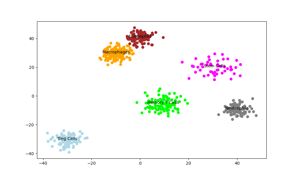
QSAR of Small Molecule Drugs: The Use of Neural Networks Quantitative Structure-Activity Relationships (QSAR), the cornerstone of modern drug discovery, has relied on linear models to predict drug activity based on molecular structure. While this has had its benefits, neural networks -particularly Graph-based Neural Networks (GNNs) like Graph Convolutional Networks (GCNs) and Graph Attention Networks (GATs) – are showing promise at capturing complex, non-linear relationships within molecular data. By learning directly from raw molecular structures, neural networks can reveal subtle patterns and interactions that simpler models might miss. In this article, we look at how GNNs represent a powerful tool in QSAR analysis. QSAR in Drug Discovery: Modeling Molecular Complexity QSAR is the process of leveraging computational modeling techniques to predict the biological activity of chemical compounds based on their structural properties. The process begins with a vast chemical database of millions of molecules, as the initial pool for potential drug candidates and these chemical structures are then converted into numerical representations called chemical descriptors, which capture various molecular properties and features. The heart of QSAR lies in its predictive models, which establish correlations between these chemical descriptors and the compound’s biological activity or property of interest. These models act as a filter, enabling virtual screening of the enormous chemical libraries. The virtual screening process efficiently narrows down the vast chemical space to a manageable set of compounds that are likely to exhibit the desired activity. This approach significantly reduces the need for extensive and costly experimental testing, as it identifies “confirmed actives” (potentially therapeutic) and “confirmed inactives” (non-toxic) compounds with higher precision. At a more granular level, QSAR modeling involves a direct relationship between compound structures and their quantitative activity measures. Molecular structures, often represented as 2D sketches or more complex 3D conformations, are systematically analyzed to extract relevant descriptors. These descriptors might include physicochemical properties, topological indices, or electronic parameters. The activity data, typically expressed as numerical values (e.g., IC50, Ki, or other standardized measures), are then correlated with these descriptors to build predictive models. The representation of chemical structures in computational systems is crucial for effective QSAR modeling. Molecules are commonly depicted as graphs, where atoms serve as vertices and chemical bonds as edges. This graph-based representation allows the calculation of numerous molecular indices and descriptors, which form the basis for quantitative comparisons between different compounds. The molecular information is often stored in specialized file formats, such as MOL files, which contain detailed information about atomic coordinates, bond types, and connectivity tables. In the realm of advanced QSAR techniques, compounds are conceptualized as vectors in a multidimensional descriptor space. Each dimension in this space corresponds to a specific molecular descriptor or property. For instance, a compound M might be represented by a vector RM = RM(xM1, xM2, …, xMK), where each xMi represents a distinct molecular feature. This vectorial representation enables researchers to quantify similarities between compounds, identify structural patterns correlated with activity, and make predictions about the properties of novel, untested compounds. This multidimensional approach thus forms the foundation for many modern QSAR methodologies. Samples (Compounds) Variables (descriptors) Compound X₁ X₂ … Xₘ 1 X₁₁ X₁₂ … X₁ₘ 2 X₂₁ X₂₂ … X₂ₘ … … … … … n Xₙ₁ Xₙ₂ … Xₙₘ This coordinate matrix enables multidimensional descriptor spaces of QSAR modeling. Here, researchers can examine how molecules form distinct clusters based on their chemical properties and structural similarities. This clustering phenomenon is visually represented as a three-dimensional space where each axis corresponds to a different molecular descriptor. Within this space, molecules with similar characteristics tend to group together, forming discrete clusters. This clustering concept is fundamental to understanding the distribution of compounds in chemical space and has significant implications for drug discovery and QSAR modeling. The dimensions of this space are determined by the number of descriptors used in the analysis, which can range from a few to hundreds or even thousands. Clustering methods are employed to analyze the distances between compounds in this multidimensional space, allowing researchers to identify groups of structurally or functionally similar molecules. This approach not only aids in the classification of known compounds but also helps in predicting the properties of new, untested molecules based on their proximity to existing clusters. QSAR modeling remains incredibly challenging due to the vast diversity of molecular structures and their corresponding biological activities. Moreover, the risk of overfitting, where a model becomes too tailored to the training data and performs poorly on new data, poses a significant obstacle. This is especially problematic in drug discovery, where models must generalize well to predict the efficacy and safety of novel compounds. Addressing these challenges requires careful model selection, robust validation techniques, and a deep understanding of both chemistry and biology. Understanding Graph-Based Neural Networks: Advancing Beyond Linear QSAR Models So we understand how modern QSAR modeling relies heavily on ‘capturing’ the chemical structure interrelationships. Technically, these can be quite easily modeled as multivariate linear regressions, known as linear QSAR models. These models assume a straightforward linear correlation between molecular descriptors (such as physicochemical properties, topological indices, and electronic parameters) and biological activity, offering simplicity, interpretability, and computational efficiency. The basic form of these models are; Y = a0 + a1X1 + a2X2 + … + anXn, where Y represents biological activity and X1, X2, etc., are molecular descriptors. However, they face significant challenges in capturing the full complexity of structure-activity relationships which tend to be nonlinear in nature. As a result they are widely used in early-stage drug discovery and toxicity prediction. However, if you are going deeper, you need to model accounting for more complexity. Enter GNNs. GNNs represent a flagship advancement in QSAR modeling because unlike traditional neural networks that operate on fixed-size inputs, GNNs are designed to process and learn from graph-structured data directly. In order to examine this let take a look at a typical architecture of a GNN: Node Embedding: Initial features are assigned to each atom (node) in the molecular graph. These could include atomic properties like
HMMs vs MSMs: Divergent Applications in Bioinformatics and Cheminformatics

HMMs vs MSMs: Divergent Applications in Bioinformatics and Cheminformatics From decoding the hidden messages in DNA to predicting the fluid motions of proteins, mathematical models serve as a lens into the microscopic world. This exploration delves into the power of Markov-based models – Hidden Markov Models and Markov State Models, revealing how these tools are used in bioinformatics and cheminformatics. Hidden Markov Models: Decoding Nature’s Discrete Cipher For example, consider a simple weather model. The hidden states are “Rainy” and “Sunny,” representing the actual weather conditions we can’t directly observe. The observable outputs are “Wet Ground” and “Dry Ground,” which we can see and measure. This model illustrates the core components of an HMM: hidden states (the true weather), observations (the ground’s moisture level), and probabilities connecting them. The power of HMMs lies in their ability to infer these hidden states from observable data, making them invaluable in deciphering complex patterns in seemingly random sequences. Hidden State Observable Output Probability Rainy Wet Ground 0.8 Rainy Dry Ground 0.2 Sunny Wet Ground 0.1 Sunny Dry Ground 0.9 In bioinformatics, HMMs find extensive application in gene prediction. The power of HMMs in this context lies in their ability to capture the inherent structure of genes without explicit programming of biological rules. The model learns to identify coding and non-coding regions in DNA sequences by recognizing subtle patterns in the nucleotide composition and order. Position Observed Base Hidden State 1 (5′ end) A Coding 2 T Coding 3 G Non-coding 4 (3′ end) C Non-coding … … … As the HMM moves along the DNA sequence from the 5′ to 3′ end (the conventional direction for reading DNA, where 5′ and 3′ refer to the carbon atoms in the sugar-phosphate backbone), it predicts the most likely hidden state (coding or non-coding) for each observed base. Once trained on reference genomes, the HMM can be applied to novel, unannotated sequences to predict gene structures. This allows researchers to identify potential genes in newly sequenced organisms or find previously unrecognized genes in well-studied genomes. The HMM’s ability to generalize from training data makes it a powerful tool for comparative genomics and the discovery of conserved genetic elements across species. The HMM learns transition probabilities between states (e.g., the likelihood of transitioning from a coding to a non-coding region) and emission probabilities of bases in each state (e.g., the frequency of each nucleotide in coding vs. non-coding regions). This probabilistic approach allows HMMs to capture complex biological phenomena, such as: Splice site recognition: HMMs can identify the boundaries between exons and introns by learning the specific nucleotide patterns associated with splice sites. Gene structure variation: The model can adapt to different gene structures, including alternative splicing, by learning multiple paths through the state space. Species-specific patterns: HMMs can be trained on species-specific data, capturing the unique genomic characteristics of different organisms. Handling ambiguity: The probabilistic nature of HMMs allows them to manage the inherent uncertainty in biological sequences, making them robust to sequencing errors and natural variations. This flexibility and ability to capture complex patterns make HMMs particularly powerful in genomic analysis, enabling accurate gene prediction in unknown sequences across diverse species. Markov State Models: Navigating the Molecular Continuum While HMMs excel in bioinformatics, its cousin, Markov State Models (MSMs), find greater application in cheminformatics, particularly in molecular dynamics simulations. This divergence stems from the fundamental differences in the systems they model. MSMs handle directly observable states and are adept at analyzing continuous state spaces, making them ideal for the complex, fluid world of molecular interactions. The limited use of HMMs in cheminformatics is rooted in the nature of molecular systems. These systems often exhibit continuous conformational spaces, which HMMs, with their discrete state representations, struggle to capture efficiently. For example, consider a protein folding process. While an HMM might represent the protein as either “folded” or “unfolded,” the reality involves a continuum of intermediate states. An MSM can more accurately represent this by discretizing the continuous space into numerous microstates, each representing a small region of the conformational landscape. Moreover, the computational intensity of HMMs becomes prohibitive for large-scale molecular simulations, where MSMs offer a more scalable approach. MSMs solve this by allowing the construction of a model from multiple, shorter simulations rather than requiring a single, long trajectory. This “divide and conquer” approach significantly reduces computational demands while maintaining accuracy. Crucially, MSMs naturally incorporate time reversibility, meaning the probability of transitioning from state A to B is the same as B to A when the system is at equilibrium. This property aligns with the physical reality of many chemical processes, where microscopic reversibility is a fundamental principle. For instance, in protein-ligand binding, the rates of association and dissociation are related through equilibrium constants, a concept naturally captured by MSMs but not inherently represented in HMMs. In conformational analysis, MSMs excel at identifying stable states and transition pathways in protein-ligand interactions, providing a nuanced understanding of molecular recognition processes. This capability extends to estimating binding kinetics, where MSMs can predict kon and koff rates for drug-target interactions, offering critical information for drug efficacy and residence time. As a result of all these domain advantages, MSMs have proven instrumental in explaining allosteric mechanisms, capturing the subtle, long-range conformational changes that underpin many protein functions. This ability to model complex, spatially distributed phenomena makes MSMs particularly valuable in understanding the dynamic behavior of proteins and their interactions with small molecules, thereby guiding rational drug design efforts. Hybrid Markov Models: Bridging Discrete and Continuous Domains Increasingly, researchers are exploring hybrid approaches that combine elements of both HMMs and MSMs. Hybrid approaches like semi-Markov models are emerging as powerful tools in drug discovery, offering enhanced flexibility over traditional Markov models. Unlike standard Markov models, which assume a constant probability of transitioning between states regardless of time spent in the current state, semi-Markov models allow transition probabilities to depend on the sojourn time. This feature is crucial for modeling complex biological processes and pharmacokinetics where the timing of state
LLMs in Investment Research (I) – The Excel Enigma

neuralgap.io Home Sentinel Articles Home Sentinel Articles LLMs in Investment Research (I) – The Excel Enigma Despite the remarkable strides LLMs have demonstrated, deciphering the complex world of financial excel models has still been a formidable challenge. The structured, data-rich environment of spreadsheets, particularly those used in financial modeling, presents a unique set of obstacles that push the boundaries of what LLMs can currently achieve. At first glance, an excel spreadsheet might seem simpler to process than a lengthy text document because it’s just rows and columns of data. But for an LLM, which was primarily trained on natural language, interpreting a financial model is akin to reading a foreign language written in a three-dimensional, interconnected script. In this article we dive into why these types of data remain a challenge and how we can overcome them. Complexity of Linkages The first hurdle LLMs encounter is the complex structure of financial models. Unlike linear text, these spreadsheets are often sprawling ecosystems of multiple interconnected sheets. Each cell can be a world unto itself, hosting formulas that reference data across different sheets and even different files. The hierarchical nature of financial statements – where an income statement feeds into a balance sheet and cash flow statement – adds yet another layer of complexity. For an LLM, understanding these intricate relationships is like trying to map a city by looking at it through a keyhole. Formula comprehension Formula comprehension presents another significant challenge. Financial Excel models are often built on a foundation of complex formulas, ranging from nested IF statements to array formulas and financial functions like NPV and IRR. These aren’t just calculations; they’re the DNA of the financial model, encoding business logic, assumptions, and financial principles. An LLM needs to not only parse the syntax of these formulas but also grasp their financial implications and how they contribute to the overall model structure. It’s not enough to know what a VLOOKUP does; the model needs to understand why it’s being used and what its output signifies in the broader financial context. Temporal Nature of Data The variability of data types within a single model further complicates matters. Each data type comes with its own rules and conventions. An LLM must correctly identify and interpret these different data types, especially when they’re used together in calculations. For instance, Is a number a dollar amount or a ratio? Is it a date at the end of a fiscal year or a loan maturity? These distinctions are second nature to a human financial analyst but require sophisticated understanding from an AI model. Moreover, one of the most challenging aspects for LLMs is dealing with the temporal nature of financial models. Many spreadsheets are structured with columns representing different time periods – months, quarters, or years. Understanding these temporal relationships and how they affect calculations, such as year-over-year growth or cumulative totals, is crucial. An LLM needs to develop a sense of financial time, recognizing how past, present, and projected future data interact within the model. Size and Added Feature Complexity As we delve deeper into the world of financial modeling, we uncover even more complex features that push the limits of current LLM capabilities. Named ranges, custom functions, circular references, and scenario analyses are just a few of the advanced Excel techniques that are commonplace in sophisticated financial models. Each of these features requires not just technical understanding but also an appreciation of their purpose and implications in financial analysis. The sheer scale of many financial models presents another significant hurdle. It’s not uncommon for these spreadsheets to contain thousands of rows of data across multiple sheets. This volume of information stretches the processing capabilities of LLMs, which often struggle with very long input sequences. How can an AI model maintain context and accuracy when dealing with such vast amounts of interconnected data? In essence, interpreting a financial Excel model requires more than just processing rows and columns of data. It demands an understanding of financial principles, Excel-specific features, industry conventions, and the ability to follow complex logical and mathematical relationships across a multidimensional structure. For LLMs, mastering this challenge is not just about improving their ability to handle structured data – it’s about developing a form of financial literacy and Excel fluency that rivals that of human experts. In our next set of articles we are going to navigate how we address each of the above (at least partially) for LLMs. Stay tuned! Looking to integrate AI into your Research? Our flagship product Sentinel is designed to be and end-to-end platform that helps Investment Research companies 2x their productivity. Please enable JavaScript in your browser to complete this form.Please enable JavaScript in your browser to complete this form.Name *Email *Organization/Institution * What products/subscriptions do you currently use? * Bloomberg/Factset AlphaSense Morningstar Other (please specify): Which processes do you want to streamline? * Financial modelling Primary Research Secondary Research Quality Checking Other Let us know if you have any questions! Submit ©2023. Neuralgap.io
Transformers in Biotech (I) – How it Started
Transformers in Biotech (I) – How it Started Transformer models have emerged as a powerful tool in various domains of AI, particularly in natural language processing, and more recently, bioinformatics. Transformers were originally introduced in the paper “Attention is All You Need” by Vaswani et al. in 2017, and rely on a mechanism called “self-attention” to process input data allowing them to handle sequential data, capture long-range dependencies, and manage large datasets efficiently. This naturally makes them a great fit for bioinformatics applications, especially sequencing and structure predictions. In essence, transformers work by paying attention to different parts of the input data simultaneously, which is a departure from the traditional recurrent neural networks (RNNs) that process data sequentially. This parallel processing capability not only speeds up training but also enables transformers to achieve superior performance on many complex tasks. Their architecture consists of an encoder and a decoder, both made up of multiple layers of self-attention and feedforward neural networks. In this article series, we will be examining transformer variants across the spectrum of bioinformatics, and examining them in 3 parts: Structural Biology Transformers for analyzing amino acid sequences and predicting 3D protein structures Models to look at include AlphaFold and OmegaFold NLP Transformers for Biomedical text mining, disease detection, risk factor extraction, and clinical decision support Models to look at include BioBERT, InferBERT, and BioGPT Medical Imaging Vision Transformers for Medical image segmentation, predicting tissue regions and structures, and enhancing image resolution for better diagnosis Models to look at include HisTogene But first, let’s have a brief run through of how we got here. for analyzing amino acid sequences and predicting three-dimensional protein structures First uses of transformers in bioinformatics Even a decade earlier, transformers were proposed in research as a potential solution to long sequencing problems in bioinformatics, but it is in 2019 when we started seeing research articles pop up with its applications. Papers such as “Predicting multiple cancer phenotypes based on somatic genomic alterations via the genomic impact transformer” by Yifeng Tao, Chunhui Cai, William W. Cohen, and Xinghua Lu and “Novel transformer networks for improved sequence labeling in genomics” by Jim Clauwaert and Willem Waegeman, revised and published towards late 2019, are classic examples of these. These papers discussed the benefits of applying multi-headed attention in long sequences, emphasizing the introduction of transformer architectures for whole-genome sequence labeling tasks, showing state-of-the-art performances and unbiased benchmarking results. This research interest was primarily fueled by the promising results of Open AI’s GPT 2 which was also released in late 2019. One of the first successful implementations of transformers was in early 2021 with the introduction of DNABERT. This model adapted the BERT architecture to understand and process DNA sequences by pre-training on a human reference genome using k-mer tokenization. DNABERT demonstrated significant improvements in tasks such as DNA sequence classification and motif prediction, paving the way for more sophisticated analyses in genomics using transformer models. Meanwhile, research rapidly became more nuanced and insightful. For example, in March 2021, the paper TALE: Transformer-based protein function Annotation with joint sequence-Label Embedding by Yue Cao and Yang Shen was published in Bioinformatics which highlights the use of transformers for protein function annotation by leveraging joint sequence-label embedding to improve functional insights from high-throughput sequence data. Naturally, explainability started becoming a prominent requirement. Studies such as the Explainability in transformer models for functional genomics by Jim Clauwaert, Gerben Menschaert, and Willem Waegeman, published in Briefings in Bioinformatics, showed the potential for unveiling the decision-making process of trained models. This also emphasized the need for new strategies to benefit from automated learning methods by revealing the decision-making process, specifically focusing on the automatic selection of relevant nucleotide motifs from DNA sequences. Transformer Architecture in Genomics: A Closer Look To better understand why transformers are particularly well-suited for genomic data analysis, let’s examine a specific implementation in detail. We’ll narrow our focus to a paper titled Transformer-based genomic prediction method fused with knowledge-guided module. This case study will allow us to highlight the key features that make transformer architectures so powerful in the field of genomics. By breaking down the components of this transformer-based genomic prediction method, we can illustrate how these models adapt to the unique challenges of biological sequences. Implementing Transformers for Genomic Data: A Case Study in Sequence Analysis The implementation of an “LLM-like” transformer model – but for genomic data – leverages the transformer architecture’s ability to handle both sequential and non-sequential data. Key to this process is tokenization, where sequential data, like DNA sequences, are converted into k-mers, while non-sequential data, such as single-cell RNA-seq, use gene IDs or expression values as tokens. Crucially, positional encoding is applied to these tokens to preserve the sequential information in genomic data. This is especially important for understanding the relative positions of genetic elements, which can significantly impact function. The transformer models employ masked language modeling (MLM) during pre-training, where tokens are masked, and the model predicts them using context from surrounding tokens. This enables the model to capture complex patterns and relationships within genomic data. The self-attention mechanism in transformers facilitates the model’s ability to attend to long-range dependencies, crucial for understanding genomic sequences that can span thousands of base pairs. By using multi-head attention, the models can jointly focus on different subspaces of the input, enhancing their predictive power. The final layers, including add-and-norm layers and fully-connected layers, refine these predictions, enabling the model to make accurate predictions on functional regions, disease-causing Single Nucleotide Polymorphisms (SNPs), and gene expression levels. Explainability in Genomic Transformers: Examples from Recent Research Explainability is crucial in bioinformatics, as researchers need to understand the decision-making process that leads to specific outputs. In a recent application of transformers to genomic data, researchers employed two key methods to enhance model interpretability: Layer-wise Relevance Propagation (LRP): This technique decomposes the model’s prediction, assigning importance scores to individual input features. It works by redistributing the prediction score backward through the network layers. In the context of genomic data, LRP
When is Big Data Big?

neuralgap.io Dawn Articles Dawn Articles When is Big Data Big? The term “big data” has historically been encapsulated by the three Vs: Volume, Velocity, and Variety. Volume refers to the sheer amount of data being generated and stored; it’s the most apparent characteristic that defines data as “big.” Velocity denotes the speed at which new data is produced and the pace at which it moves through systems. Variety speaks to the diverse types of data, from structured numeric data in traditional databases to unstructured text, images, and more. These dimensions have served as a foundation for understanding the challenges and opportunities inherent in managing large datasets. A Quick Recap Let’s put this into perspective, by considering a naive range between 100,000 data points, which might represent a modest dataset by today’s standards, and 1 billion data points, a volume that challenges even sophisticated analysis tools and storage systems. This vast range highlights the practical implications of big data: as datasets grow from one end of the spectrum to the other, the complexity of processing, analyzing, and deriving insights increases exponentially, necessitating more advanced computational techniques and infrastructures. For the context of the rest of this article – we are going to assume that you already have basic knowledge about data and its attributes. Real-World Nuances: Why definition is difficult Big data’s complexity extends far beyond its volume, challenging our traditional understanding and approaches. Two critical aspects that significantly influence data management and analysis strategies are high dimensionality and data sparsity. High Dimensionality: Challenges and Implications High-dimensional data spaces, where datasets contain a vast number of attributes or features, present unique challenges. As the dimensionality increases, the data becomes more sparse, making it difficult to apply conventional analysis techniques due to the “curse of dimensionality.” This phenomenon not only complicates data visualization and interpretation but also requires sophisticated algorithms for pattern recognition and predictive modeling. Managing such datasets demands significant computational resources and innovative data processing strategies to extract meaningful insights without getting lost in the sheer complexity of the data structure. Sparse Data: Understanding the Impact Sparse data, where the majority of elements are zeros or otherwise lack significant value, poses its own set of challenges. In contexts where data sparsity is prevalent, such as in large matrices in recommender systems or genomic data, storage efficiency and data processing speed become critical concerns. Techniques like compression and the use of specialized data structures become essential to manage and analyze sparse data effectively, ensuring that computational resources are not wasted on processing large volumes of non-informative data. Intensive Data Operations: Certain data operations inherently feel “big” due to the intensity and computational demands they impose. Operations like semantic search, which requires understanding the context and meaning behind words and phrases, exemplify how data’s complexity can make it feel large. These operations often require advanced AI and machine learning algorithms to process data efficiently, highlighting the significance of computational techniques in managing the perceived bigness of data. Algorithmic Complexity: The complexity of algorithms, particularly those with O(n^2) time complexity like nearest neighbor searches, significantly impacts how we manage and analyze big data. These algorithms become impractically slow as the dataset grows, illustrating a crucial aspect of big data challenges—the interplay between data size and algorithmic efficiency. Innovations in algorithm design, such as approximation algorithms and efficient indexing techniques, are vital for mitigating these challenges, enabling faster data processing and analysis even as datasets continue to expand. Data Quality and Cleanliness: The Hidden Costs and Challenges Ensuring data quality and cleanliness becomes exponentially more difficult as datasets grow. Issues such as incomplete records, inaccuracies, duplicates, and outdated information can severely impact the insights derived from big data. Challenges with Setting Up an ETL Pipeline: Establishing an efficient Extracting, Transforming, and Loading (ETL) pipeline presents numerous challenges, especially when dealing with big data. The pipeline must be designed to handle the vast volume of data constantly and efficiently, ensure the integrity and cleanliness of the data throughout the process, and be flexible enough to accommodate changes in data sources and formats. Take as an example a healthcare dataset with 10 million patient records. In this dataset, suppose that 0.5% of the records contain critical inaccuracies in patient diagnosis codes, and 2% of records are duplicates due to patients receiving care at multiple facilities within the same network. These issues, although seemingly small in percentage terms, translate to 50,000 records with incorrect diagnoses and 200,000 duplicate records, however the transform process required to solve this still is required to sift through all 10 million of the dataset just to catch those (and avoid Type II errors, also known as false negatives). Timing and activity synchronization: One of the more subtle yet pervasive challenges in managing global datasets is timing and activity synchronization. This issue arises from the need to accurately align and interpret timestamped data collected from different time zones. For instance, a purchase made at 12 AM in New York (GMT-4) corresponds to 9 AM in Tokyo (GMT+9). Without proper synchronization, activities that span multiple time zones can lead to misleading analyses, such as underestimating peak activity hours or misaligning transaction sequences. To address this, data engineers must implement robust time synchronization techniques that account for the complexities of global timekeeping, such as daylight saving adjustments and time zone differences. This might involve converting all timestamps to a standard time zone, like UTC, during the ETL process, and ensuring that all data analysis tools are aware of and can correctly interpret these standardized timestamps. However, even with these measures, challenges persist in ensuring that time-sensitive data analyses accurately reflect the intended temporal relationships and behaviors. Data Aging and Historical Integrity: Data aging refers to the process by which data becomes less relevant or accurate as time passes, potentially leading to misleading conclusions if not managed properly. Maintaining historical integrity involves not just preserving data but also ensuring it remains meaningful and accurate within its intended context (remember, archiving data is also expensive and accumulative).
Setting up a Data Exploration Team: Part II

neuralgap.io Dawn Articles Dawn Articles Setting up a Data Science Team: Part II Building on the foundational steps established in Part I, this section delves into the operational aspects of implementing a data science strategy within an organization. It encompasses selecting appropriate tools and infrastructure, optimizing workflow and processes for efficiency and agility, and assembling a team with a diverse range of skills and expertise. These elements are crucial for translating strategic objectives into actionable insights and innovations, further cementing data science’s role as a key driver of business success. We will explore the nuances of tooling and infrastructure choices, the dynamics of data science project lifecycles, and the composition and roles within an effective data science team. Tooling and Infrastructure Choosing the right tools and technologies for a data science team involves a careful consideration of the team’s expertise, the organization’s existing technological ecosystem, and the specific requirements of data science projects. Lets try to elaborate with a few common use cases and scenarios. Relevant data analysis software is essential, for example, R Studio is particularly beneficial for teams with strong statistical analysis backgrounds, ideal for complex data modeling and visualization projects, whereas Tableau is best suited for teams focused on business intelligence and data visualization, allowing non-technical stakeholders to understand data insights easily (perhaps assuming your data is already well organized or doesn’t require that much effort to organize). Cloud platform selection is often dictated by the organization’s existing architecture and compatibility requirements. Very generally speaking, AWS offers a broad set of tools and services with granular control, Google Cloud Platform for robust ease of set up and use and Microsoft Azure for organizations already heavily invested in Microsoft products, as it seamlessly integrates with the broader ecosystem (we are going to leave aside the discussion of ‘On-premise vs. Cloud’ for a later article). Skill set weighting programming languages, to a lesser degree, also contribute to success. Today, mostly Python is the go-to tool given its versatility, due to its robust data manipulation, and machine learning libraries. In contrast R is still preferred for teams specialized in statistical analysis and academic research. Other (not strictly programming languages) like knowledge in SQL will be essential for efficient data retrieval and manipulation. Workflow and Processes It goes without a saying that efficient workflows and processes are the backbone of successful data science projects, so let’s try to illustrate with a few examples and some context. Setting up a clear data science project lifecycle encompasses several stages starting with: Data collection, where diverse data sources are identified and gathered. Data cleaning and preparation follow, involving the removal of inaccuracies and inconsistencies to ensure the quality of the data set. Exploratory data analysis, where patterns and insights are identified, leading to the development and training of machine learning models. Evaluation for their performance and deployed into production, where they can provide actionable insights or automate decision-making processes. Agile Methodologies in Data Science means adapting quickly to changing requirements or new insights. Sprint Planning: Defining short, manageable phases of work, allowing for rapid adjustments and focused efforts on high-priority tasks. Stand-ups: Regular short meetings to update the team on progress, obstacles, and next steps, ensuring alignment and facilitating problem-solving. Retrospectives: Reflecting on the completed work to identify successes and areas for improvement, driving incremental enhancements in processes and outcomes. Collaboration between Data Science and Other Departments (such as IT and business units) is crucial for aligning data science projects with business objectives and operational capabilities. Let’s try to paint a clear picture by using examples of what NOT to do in each. Not understanding the core KPIs to be tracked – a classic sign of insufficient communication between departments. Providing or extracting overwhelming ‘information’ – a sign of departments not knowing what is useful information. Lack of Synchronization on project goals – when projects are initiated without a clear, shared understanding of the expected outcomes, e.g., IT department deploys infrastructure that prioritizes data security over accessibility, it can hinder the data science team’s ability to quickly iterate on models. Failure to establish feedback loops – e.g., a data science team proceeding to develop and refine a model for months without checking in with business stakeholders, only to find out that market conditions have changed, and the model no longer addresses the most pressing business needs. Workflow and Processes Given the complexities and strategic importance of data science initiatives, as outlined in our discussions on tooling, infrastructure, workflow, and processes, the composition of the data science team becomes paramount. The roles within the team are not just job titles but define the capabilities, innovation, and execution power of the entire operation. Lets take a look at a few common roles. Data Scientists: Specialists who analyze and interpret complex digital data, such as the usage statistics of a website, especially in order to assist a business in its decision-making. They bring statistical modeling knowledge and the ability to leverage data in strategic decision-making. Data Engineers: Responsible for preparing the ‘big data’ infrastructure for analysis. They focus on the design, construction, and maintenance of the systems that allow data to be accessed and stored effectively. Data Analysts: Focus on processing and performing statistical analysis on existing datasets. They help in interpreting the data, turning it into information which can offer ways to improve a business, thus affecting business decisions. Machine Learning Engineers: Specialize in writing software to make computers and machines operate without being explicitly programmed for specific tasks. They create algorithms that allow software to become more accurate in predicting outcomes without being specifically programmed. In reality a lot of the roles have significant overlaps with each other and are used differently in different industries. Regardless, the core skill sets required remain the same. Also a quick note about domain experts. Domain experts help to guide the data science process from hypothesis formation to model interpretation in a way that aligns with specific business objectives and industry nuances. For example, in healthcare, a data
Setting up a Data Exploration Team: Part I

neuralgap.io Dawn Articles Dawn Articles Setting up a Data Science Team: Part I Embarking on the journey to establish a data science team and strategy requires setting clear objectives, a thorough understanding of the available data, and the right mix of talent. This guide outlines the foundational steps for organizations aiming to harness data science: setting precise goals that align with business ambitions, navigating the complexities of data infrastructure and governance, and assembling a team equipped with diverse expertise. Together, these components are critical for transforming raw data into strategic insights, positioning data science as a pivotal force in driving organizational success. Defining Your Insight Generation Objectives The first step in defining data science objectives is to identify the overarching business goals. This involves understanding what the business aims to achieve in both the short and long term. Objectives can range from increasing revenue, reducing costs, enhancing customer satisfaction, to streamlining operations. It’s crucial to align data science projects with these goals to ensure that the efforts contribute directly to the company’s success. This alignment involves stakeholders from relevant departments to articulate and agree upon clear, measurable outcomes that data science initiatives aim to support. Measuring business objectives involves establishing Key Performance Indicators (KPIs) that are specific, measurable, achievable, relevant, and time-bound (SMART). For instance, if the objective is to enhance customer satisfaction, a relevant KPI could be the Net Promoter Score (NPS). If the goal is to increase revenue, a KPI might be monthly sales growth. Data science projects should aim to move these KPIs in the desired direction, and thus, the success of these projects can be evaluated based on their impact on the KPIs. Regular monitoring and reporting of these indicators ensure that the team remains focused and can adjust strategies as needed. Let’s consider a client in the payables/merchant transactions sector. Their business objectives might include reducing transaction processing times, decreasing the rate of fraudulent transactions, and increasing customer retention rates. Objective 1: Reduce Transaction Processing Time Measure: Average processing time per transaction. Data Science Application: Implement machine learning algorithms to predict and prioritize transactions based on risk, speeding up low-risk transactions. Objective 2: Decrease Fraudulent Transactions Measure: Percentage of transactions identified as fraudulent. Data Science Application: Develop a fraud detection system using anomaly detection techniques to identify patterns indicative of fraud. Objective 3: Increase Customer Retention Rates Measure: Customer churn rate. Data Science Application: Use predictive analytics to identify customers at high risk of churning and develop targeted interventions to improve retention. Understanding Your Data Landscape Once clear and compelling goals have been established, the next critical step in the data science process is to thoroughly analyze your data landscape. This analysis involves a comprehensive review of the current state of your data infrastructure, understanding and implementing robust data governance policies, and identifying the various sources of data available. This foundation is essential for ensuring that your data science initiatives are built on a solid, reliable base. Evaluating your data infrastructure involves examining the systems and technologies in place for collecting, storing, processing, and accessing data. Key aspects to consider include the scalability, reliability, and efficiency of data storage solutions, the availability of data processing and analytics tools, and the integration capabilities between different data sources and systems. This assessment helps identify potential bottlenecks, data silos, or outdated technologies that may hinder data science projects, guiding necessary upgrades or changes to support more sophisticated data analysis and machine learning efforts. A couple of examples would be Data Storage Solutions: Relational Databases: MySQL, PostgreSQL, Oracle – for structured data with robust querying. NoSQL Databases: MongoDB, Cassandra, DynamoDB – for flexible and scalable unstructured data. Data Processing and Analytics Tools: Apache Spark: A comprehensive engine for big data processing with libraries for SQL, machine learning, and more. Apache Hadoop: Framework for distributed processing of large data sets across computer clusters. Data Integration and ETL Tools: Apache Kafka: Real-time streaming platform for data publishing, subscribing, and processing. Talend: Data integration and transformation across cloud and on-premise environments. Machine Learning and Advanced Analytics: TensorFlow, PyTorch: Libraries for machine learning and deep learning with rich ecosystems. Scikit-learn: Python library for efficient data mining and analysis. Cloud-Based Data Services: AWS, Google Cloud, Microsoft Azure: Comprehensive cloud services for data storage, processing, and analytics. Data Governance – Policies for Data Quality, Security, and Privacy: Data governance encompasses the policies and procedures that ensure high-quality, secure, and private data management within an organization. It includes establishing standards for data quality to ensure accuracy, consistency, and reliability of the data used in analysis. Security policies protect sensitive data from unauthorized access and breaches, while privacy policies ensure compliance with legal and regulatory requirements related to data protection, such as GDPR or HIPAA. Effective data governance is critical for maintaining trust in data science outcomes and ensuring ethical use of data. Sources of Data – Internal, External, Structured, and Unstructured: Understanding the variety of data sources available is crucial for leveraging the full potential of data science. Internal Data: This includes data generated from within the organization, such as sales records, customer interactions, and operational data. Internal data is often structured and stored in databases but can also include unstructured data like emails or documents. Furthermore, this includes expansion of internal data collection as required by the project, i.e. a specific Machine Learning model training would only be possible if new data or data points collected are expanded. External Data: External sources provide additional insights that complement internal data. This can include data from market research, social media, public databases, or data purchased from third-party providers. External data varies widely in structure and format, requiring effective strategies for integration and analysis. Structured Data: This refers to data that adheres to a predefined model or format, making it easily searchable and organized in databases. Examples include spreadsheets or SQL databases where each data element is clearly defined. Unstructured Data: Unstructured data lacks a predefined format, including text, images, video, and web pages. Analyzing unstructured data
Determinism II: Prompt templates and the impact on Output

neuralgap.io Dawn Articles Dawn Articles Determinism II: Prompt templates and the impact on Output LLMs are all the rage, but part of using their potency well is understanding the source of their randomness and the sensitivity of their output to their input. We will continue to explore this in our series on the Neuralgap website, that will explore further on engineering challenges on the cross-section of LLMs and Big-Data. The Source of Randomness in LLMs As we all know, Large Language Models (LLMs) like OpenAI’s GPT or Google’s Gemini all rely on the now famous architecture of Generative Pretrained Transformers which at their heart rely on next word prediction. At inference, when generating this next word your input text goes through a few layers that have pre-determined randomness injected into it. Let’s take a look at these layers in detail below. Layer 1: Random Seed Initialization At the forefront of introducing variability in LLMs is the process of random seed initialization during inference. The seed can be perceived as the starting point for the pseudo-random number generation process that underlies various stochastic operations within the model, including the aforementioned stochastic sampling. When a specific seed is used, it ensures a reproducible pattern of “randomness.” This means that for a given input and a fixed seed, the model will consistently generate the same output. This consistency is paramount for applications requiring stability and predictability. However, varying the seed, even with the same input, can lead to divergent outputs, highlighting the seed’s role in modulating the balance between consistency and variability in the model’s responses. Layer 2: Stochastic Sampling (Temperature-Based Sampling) Similarly, variability in LLMs is also affected by the process of stochastic sampling, particularly temperature-based sampling. When an LLM generates text, it computes a probability distribution for the next word based on the given context. This distribution reflects how likely each word in the model’s vocabulary is to follow the given sequence of words. The temperature parameter modulates this distribution. A ‘temperature’ in this context does not refer to physical warmth but is a metaphorical dial that adjusts the randomness in the model’s choices. At a high temperature, the probability distribution becomes ‘flatter’, meaning the differences in likelihood between words are reduced. This encourages the model to occasionally pick less likely words, adding elements of surprise or creativity to the output. At a low temperature, the distribution is ‘sharper’, with the model favoring the most likely words, thus producing more predictable and conservative text. Layer 3: Beam Search with Randomness Beam search, particularly when infused with an element of randomness, constitutes the third layer of randomness in LLMs. During inference, beam search involves exploring multiple potential paths for the next word or sequence of words, thereby expanding the range of possible outputs. When a stochastic component is integrated, such as randomly selecting from the top-rated beams, it introduces an additional layer of unpredictability. This method not only enhances the diversity of the generated text but also provides a means to escape potential local maxima in the probability landscape, enabling the model to explore more creative or less obvious textual paths. The inclusion of randomness in beam search underscores its significance in enriching the model’s generative capabilities, making it a vital tool for applications that benefit from a broader spectrum of linguistic expressions. A key point to note is that if we always start with the same seed parameter at inference – the model will generally always reproduce the exact same answer. However, we must also realize that this only solves reproducibility, but it does not solve inherent control for how an output reacts to input perturbation – i.e., how to exactly control the output given a certain input. For more insight into this we recommend you to take a look into Revisit Input Perturbation Problems for LLMs: A Unified Robustness Evaluation Framework for Noisy Slot Filling Task, and Semantic Consistency for Assuring Reliability of Large Language Models. We shall explore how we can at least tame these powerful models in the next part of our series “Determinism III: Controlling for Output Variation in LLMs” Interested in knowing more? Schedule a Call with us! At Neuralgap – we deal daily with the challenges and difficulties in implementing, running and mining data for insight. Neuralgap is focussed on enabling transformative AI-assisted Data Analytics mining to enable ramp-up/ramp-down mining insights to cater to the data ingestion requirements of our clients. Our flagship product, Forager, is an intelligent big data analytics platform that democratizes the analysis of corporate big data, enabling users of any experience level to unearth actionable insights from large datasets. Equipped with an intelligent UI that takes cues from mind maps and decision trees, Forager facilitates a seamless interaction between the user and the machine, employing the advanced capabilities of modern LLMs with that of very highly optimized mining modules. This allows for not only the interpretation of complex data queries but also the anticipation of analytical needs, evolving iteratively with each user interaction. If you are interested in seeing how you could use Neuralgap Forager, or even for a custom project related to very high-end AI and Analytics deployment, visit us at https://neuralgap.io/ Please enable JavaScript in your browser to complete this form.Please enable JavaScript in your browser to complete this form. Name * FirstLast Email *Phone NumberOccupation *Primary Purpose for Using Forager Submit