Chemical Library Biases in AI-Driven Virtual Screening
Chemical Library Biases in Virtual Screening From Historical Constraints to Data Quality Understanding AI in Virtual Screening Series Continuing our exploration of challenges in AI-driven virtual screening, we now turn to the fundamental impact of chemical library composition on AI model performance and reliability. While previous discussions have focused on protein and ligand representation challenges, the inherent biases and limitations in chemical libraries themselves create distinct obstacles for AI systems attempting to navigate drug-like chemical space. From systematic biases in scaffold representation to quality variations in experimental data, these library-level challenges fundamentally shape how AI models learn and predict molecular behavior. In this third article of our series, we examine how chemical library composition affects AI model development and performance. We explore how historical biases in library construction, limitations in chemical space sampling, and data quality considerations create complex challenges for AI-driven virtual screening. Our analysis spans multiple interconnected issues: from scaffold bias and dataset homogeneity to synthetic accessibility constraints and activity landscape uncertainty, revealing how library-level factors can profoundly impact the effectiveness of AI in drug discovery. Scaffold Bias and Molecular Framework Redundancy The pervasive challenge of scaffold bias in chemical libraries stems from the historical evolution of medicinal chemistry practices and synthesis-driven discovery approaches. Traditional drug discovery campaigns often gravitate toward well-characterized molecular frameworks that offer synthetic tractability and established structure-activity relationships, leading to an over-enrichment of certain privileged scaffolds. This systematic bias manifests in both proprietary and public screening collections, where analysis reveals that up to 70% of compounds may be derivatives of fewer than 30 core scaffolds, creating “islands” of over-sampled chemical space while leaving vast regions unexplored. The implications of scaffold redundancy extend beyond simple statistical overrepresentation, fundamentally impacting the training of AI models for virtual screening. When machine learning systems are trained on these biased datasets, they develop implicit preferences for familiar chemical frameworks, potentially overlooking novel scaffold types that could offer superior binding properties or more favorable drug-like characteristics. This training bias becomes particularly problematic when exploring new target classes or attempting to identify first-in-class molecules, where the most promising chemical matter may lie in underrepresented regions of chemical space. The challenge is further compounded by the self-reinforcing nature of scaffold bias in contemporary drug discovery. Success with certain molecular frameworks leads to increased exploration of similar chemical space, while perceived risks associated with novel scaffolds create barriers to their inclusion in screening collections. This creates a complex optimization problem for AI systems, which must learn to balance the statistical reliability of well-sampled regions against the potential rewards of exploring chemical space diversity, all while accounting for the inherent uncertainties in predictive modeling of underrepresented scaffold types. Dataset Homogeneity and Diversity Constraints The fundamental challenge of limited diversity in public chemical databases extends far beyond simple scaffold redundancy, manifesting as a complex interplay of historical biases, synthetic constraints, and screening paradigms. Analysis using advanced chemoinformatic tools, particularly through Tanimoto similarity metrics and Principal Component Analysis (PCA), reveals that major public repositories exhibit significant clustering around privileged structures, with diversity indices suggesting that vast regions of theoretically accessible chemical space remain virtually unexplored. This homogeneity creates a particularly challenging environment for AI models, which must extrapolate from densely sampled regions to predict properties in sparse or empty regions of chemical space. Despite the emergence of Diversity-Oriented Synthesis (DOS) and other innovative approaches aimed at expanding chemical diversity, public datasets remain constrained by practical limitations and historical precedent. Quantitative analysis through Cyclic System Retrieval (CSR) curves demonstrates that even supposedly diverse collections often exhibit high structural redundancy, with novel scaffolds representing only a small fraction of the total compound space. This systematic bias is particularly evident in the overrepresentation of certain heterocyclic frameworks, such as pyrimidines and pyrroles, which dominate public databases due to their established synthetic accessibility and historical success in drug discovery programs. The implications for AI-driven drug discovery are profound, as these diversity constraints create inherent limitations in model training and validation. Machine learning systems trained on such homogeneous datasets inevitably develop blind spots in their predictive capabilities, particularly when encountering structural motifs that deviate significantly from the well-sampled regions of chemical space. This challenge is exacerbated by the recursive nature of the problem – as AI models trained on limited datasets guide new compound synthesis, they risk perpetuating existing biases unless explicitly designed to promote exploration of novel chemical space. Synthetic Tractability Constraints Machine learning models in virtual screening exhibit biases such as data distribution bias, favoring synthetically accessible compounds over novel structures due to training data limitations, and feature representation bias, where molecular descriptors encode preferences for common scaffolds. Additionally, reinforcement learning bias in de novo design algorithms and evaluation metric bias further reinforce the prioritization of easily synthesizable molecules, inadvertently aligning model outputs with established synthetic methodologies. This synthetic accessibility bias manifests primarily through the overrepresentation of readily synthesizable core structures, such as benzene-based frameworks and common heterocycles, while potentially valuable but synthetically challenging molecular architectures remain underexplored in virtual screening campaigns. The ramifications of this bias extend beyond simple scaffold diversity, creating a self-reinforcing cycle in drug discovery. AI models, trained predominantly on easily synthesizable compounds, develop implicit preferences for molecular features that align with conventional synthetic routes. This leads to a paradoxical situation where virtual screening efforts, despite their theoretical ability to explore vast chemical spaces, often gravitate toward molecules that mirror existing synthetic paradigms, potentially overlooking innovative structural classes that could offer superior therapeutic properties. Activity Landscape Uncertainty and Data Quality Considerations The complexity of representing chemical space in AI-driven screening extends beyond structural and synthetic considerations into the realm of activity-structure relationships, where the phenomenon of activity cliffs creates significant challenges for predictive modeling. These abrupt changes in biological activity triggered by minor structural modifications often intersect with data quality issues, creating zones of uncertainty in chemical space representation. What appears as an activity cliff in one experimental context may manifest differently under varying assay conditions, temperatures, or protein constructs, creating a complex web
Enhancing ECG Interpretation Through Multi-Modal Integration

neuralgap.io Neo Articles Neo Articles Enhancing ECG Interpretation Through Multi-Modal Integration A Next-Generation Approach to Cardiac Diagnostics Multimodal Transformers in Diagnostic Triage Current ECG interpretation faces several well-documented challenges, as highlighted in the “Development of Interpretable Machine Learning Models” study. Their analysis revealed that even experienced interpreters can struggle with overlapping wave patterns, distinguishing between normal and atrial premature beats, and identifying fusion beats. The study used visual attention tracking to demonstrate how readers tend to overly focus on QRS complexes while potentially missing critical changes in ST segments and PR intervals. These challenges are further compounded by technical limitations including baseline wandering from patient movement and electrode contact issues, which can mask subtle but important abnormalities. AI-assisted interpretation could help address these limitations by providing consistent attention across all ECG segments simultaneously. The study demonstrated that well-trained neural networks can maintain consistent analysis of all ECG components – from PR intervals through ST segments – without the attentional biases observed in human readers. Additionally, advanced AI models have shown the ability to compensate for technical variations and equipment limitations by learning to recognize patterns even in the presence of noise and baseline variations. This suggests AI could serve as a valuable second set of eyes, helping to catch subtle abnormalities that might be missed during routine human interpretation without replacing the critical role of clinical expertise. Single Modality AI models Single modality AI models focused solely on ECG signals have demonstrated remarkable capabilities in pattern recognition over the past decade. Most of the deep learning approaches have achieved binary classification accuracies of 94-99% for various cardiac conditions, with some models performing at or above cardiologist-level interpretation for specific arrhythmias. These models excel by breaking down ECG signals into key morphological components – analyzing PR intervals, QRS complexes, and ST segments simultaneously through complex neural network architectures, as demonstrated in multiple studies using the MIT-BIH database. However, single modality approaches face significant limitations. For example, in one study, they can be fooled by subtle signal perturbations (with models showing 100% confidence in wrong classifications), struggle with technical variations in ECG recordings (showing 50-72% degradation in accuracy with powerline interference), and most critically, lack the broader clinical context that human interpreters naturally integrate. Research has shown that these models tend to overly focus on QRS complexes while potentially missing critical changes in other segments, highlighting the inherent risks of relying solely on ECG signal patterns for diagnosis. Additionally, most of these models are focused on identifying specific cardiac abnormalities rather than one model detecting multiple cardiac abnormalities. Some approaches have focused on building multiclass classifiers to detect multiple cardiac abnormalities. Their performance is bounded at 72-78% range when it comes to multi-class classification problems. The primary challenge is the presence of class imbalance in most of the dataset. Because of that feature extractor is biased towards certain classes over others. The utilization of multiple datasets with multiple downstream tasks and training them together can create a robust feature extractor. Complementing with Additional Modes While single modality ECG models have shown impressive capabilities, the inherent limitations of relying solely on ECG signals highlight the need for more comprehensive approaches. Multimodal AI architectures have emerged as a promising solution, integrating diverse data streams to mirror the multifaceted approach used in clinical diagnosis. Essentially, what we would like to do is to replicate (to a certain extent) the clinical diagnostic workflows by combining multiple concurrent data streams – from real-time physiological signals to longitudinal patient records. In AI, Multimodal learning (MML) integrates diverse data types, such as imaging, signals, genomic profiles, and electronic health records, to enhance diagnostic precision, particularly in cardiovascular abnormalities. Combining MML with multitask learning (MTL), helps address the challenges of rare conditions and enhances model performance even with limited data. However, current MML approaches face challenges, including the reliance on paired datasets and the complexity of integrating multiple modalities, which can hinder explainability. To address these challenges, Neuralgap has pioneered a novel architecture called Multi-Uni-Model (MUM) for multimodal, multitask learning. This approach demonstrates significant performance improvements in cardiovascular disease prediction while modifying for smaller models (i.e. known as learnable parameters). Our model – currently called Neo – is designed to process inputs from multiple modalities simultaneously through a by using i) modality-specific encoders for each type of data (imagine ECG and Echocardiogram), ii) shared transformer layers that process and fuse these embeddings (i.e. its searches for relationships across both these modalities) and iii) task-specific heads that generate final predictions (i.e. outputs). A high level model architecture diagram is shown in the figure below. High-level architecture of Neuralgap’s Multi-Unimodal Model Our model addresses issues like negative transfer and optimization difficulties by treating each task as an independent model with separate optimizers for task-specific and shared layers, allowing for independent updates. Our training strategy balances task updates to prevent catastrophic forgetting, using mini-batches from one task at a time and ensuring equal updates across tasks. This flexible and scalable approach facilitates the addition of new tasks or modalities without major architectural changes, enhancing diagnostic accuracy in biomedical applications. Neo’s first version has been extensively validated across major cardiovascular datasets spanning multiple modalities: Icentia 11K for beat-level ECG classification MIMIC-IV-ECG for rhythm-level analysis EchoNet-Dynamic for LVEF prediction CirCor DigiScope for murmur detection CAMUS for ultrasound segmentation The model was evaluated across 100 epochs and demonstrated superior performance compared to task-specific baselines, while maintaining lower computational complexity. Our architecture also underscores the advantages of shared embeddings in recognizing underlying patterns across biosignals, medical images, medical videos, and bio audio. Its adaptability and versatility are evident in implementing various cardiovascular analysis tasks using a unified model. For example, Neo can handle complex tasks like identifying heart chamber boundaries in ultrasound images and calculating how well the heart is pumping (ejection fraction) – tasks that typically require separate specialized systems. This demonstrates the model’s ability to adapt to different types of cardiovascular assessments while maintaining accuracy. The Multi-Uni-Model (MuM) represents significant
Ligand Representation Challenges in AI scoring
Ligand Representation Challenges in AI Scoring From Chemical Space to Binding Reality Understanding AI in Virtual Screening Series Continuing our exploration of challenges in AI-driven virtual screening, we now turn to the equally critical ligand-side representation problems. While protein dynamics present one facet of the challenge, the representation of small molecules introduces its own set of complex computational hurdles. These range from capturing conformational flexibility and stereochemical complexity to addressing systematic biases in compound libraries. The integration of these ligand-specific challenges with protein representation problems creates a multidimensional optimization challenge that continues to test current deep learning architectures. In this second article of our series, we examine how machine learning approaches must navigate the vast chemical space while accurately representing molecular dynamics and structural diversity. At its core, successful ligand representation requires simultaneous consideration of multiple hierarchical features – from atomic coordinates to ensemble properties – while accounting for library-wide biases and chemical space coverage limitations. Our analysis explores how these interconnected challenges manifest across different scales of molecular complexity, from basic conformational flexibility to systematic biases in screening collections. Structural Diversity and Flexibility The fundamental challenge of representing ligand structures in machine learning models stems from their inherent structural diversity and conformational flexibility. Even seemingly simple organic molecules can adopt multiple conformations, creating a vast landscape of possible 3D arrangements that must be considered during virtual screening. This conformational flexibility spans multiple scales – from simple bond rotations to complex folding patterns in larger molecules – and creates a combinatorial explosion of possible states that AI systems must learn to navigate effectively. The representation challenge is particularly complex due to the interdependent nature of molecular movements. Individual rotatable bonds don’t operate in isolation; rather, they create coordinated patterns of movement that can dramatically alter a molecule’s overall shape and properties. This interconnectedness means that simple enumeration of possible conformers often fails to capture the true complexity of ligand behavior. Furthermore, the energy barriers between different conformational states vary widely, leading to population distributions that are highly context-dependent and influenced by factors such as solvent conditions, temperature, and binding pocket environment. Table 1 below breaks down key ligand structural features into their static and dynamic components, highlighting how each molecular element requires different mathematical frameworks for representation. This classification illustrates how seemingly simple molecular features can manifest complex dynamic behaviors that challenge traditional AI representation schemes. Table 1: How structural features (static vs. dynamic) could be represented as inputs Feature Type Static Representation Dynamic/Temporal Representation Challenges in Representation Atomic positions 3D coordinates (x,y,z) (Coordinate matrix like [[1.23, 2.45, 0.67], [2.34, 1.56, 3.78]]) Time series of atomic positions (Trajectory matrix like [[[1.23, 2.45, 0.67], [2.34, 1.56, 3.78]], [1.25, 2.48, 0.69], [2.37, 1.59, 3.82]]]) Variable atom counts, multiple stable conformers Bond rotations Torsion angle values (Angle vector like [180.0, 60.5, -60.0]) Trajectory of dihedral angles (Time series matrix like [[180.0, 60.5, -60.0], [175.3, 63.2, -58.7]]) Energy barriers between rotameric states Ring systems Fixed ring conformations (Puckering parameters like [Q=0.63, θ=12.5, φ=85.2]) Pseudorotation and ring flipping trajectories (Time series of parameters like [[0.63, 12.5, 85.2], [0.61, 14.2, 87.5]]) Multiple low-energy puckering states Overall shape Single low-energy conformer (Feature vector like [vol=245.3, SA=142.8, gyr=2.34]) Ensemble of conformational descriptors (Distribution matrix like [[245.3, 142.8, 2.34], [248.1, 144.2, 2.38]]) Balance between exhaustiveness and computational cost Chemical Space Complexity The vastness of chemical space, with over 10^60 possible drug-like molecules, presents unique representation challenges for AI systems. The core difficulty lies not just in the number of possibilities, but in how ligands interact with their targets through multiple complex mechanisms. AI models must simultaneously process rigid scaffold regions that define core binding poses, flexible linking segments that can adopt multiple conformations, and peripheral groups that fine-tune binding through subtle electronic and steric effects. Each aspect of ligand structure poses distinct computational challenges. Scaffold recognition requires AI systems to identify key pharmacophoric features while accounting for potential bioisosteric replacements – where chemically different groups can serve identical binding functions. Ring systems add another layer of complexity, as their conformational preferences can shift dramatically upon binding, requiring models to understand both inherent ring flexibility and induced-fit effects. Furthermore, the spatial arrangement of functional groups creates complex electronic fields and hydrogen bonding networks that can be highly context-dependent, varying based on local environment and protein dynamics. Table 2 breaks down these ligand-specific challenges for AI representation, highlighting how different structural elements contribute to the overall complexity of binding prediction. Table 2: How chemical spaces features (static vs. dynamic) could be represented as inputs Feature Type Static Representation Dynamic/Temporal Representation Challenges in Representation Scaffold core Single conformer graph representation (e.g., [C-C-C-N] backbone) Ensemble of accessible scaffold conformations (Multiple stable states) Core flexibility affects binding modes Functional groups Fixed functional group positions (Feature vector like [-OH, -NH2, -COOH]) Time-dependent group orientations and interactions (Rotamer distributions) Context-dependent electronic effects– Water-mediated interactions Ring systems Basic ring conformations (e.g., chair/boat forms) Dynamic ring puckering trajectories (Time series of puckering parameters) Multiple low-energy states– Ring flip barriers Molecular properties Static property vector:– LogP– Polar surface area– Molecular weight(Feature vector like [3.2, 95.6, 350]) Time-dependent properties:– Changing solvent exposure– Dynamic charge distributions– Varying H-bond networks(e.g., Time series matrices) Environmental dependencies– Conformational effects on properties Stereochemical and 3D Considerations The representation of molecular stereochemistry presents a fundamental challenge that extends beyond simple atomic connectivity. Each chiral center in a molecule doubles the number of possible stereoisomers, creating distinct three-dimensional arrangements that can dramatically affect biological activity. For instance, a molecule with three chiral centers generates eight possible stereoisomers, each potentially interacting with the target protein in fundamentally different ways. This stereochemical complexity is further amplified in molecules containing axial chirality, where restricted rotation around bonds creates atropisomers with distinct spatial orientations. Configurational stability thresholds can also be used to ignore rapidly interconverting stereoisomers at physiological temperatures. Beyond discrete stereoisomers, molecules exhibit complex shape-based properties that emerge from their three-dimensional arrangement. The accessible surface area varies dynamically as molecules rotate and flex, creating time-dependent exposure of polar and nonpolar
Computational Representation Challenges in Protein-Ligand Scoring
Protein Representation Challenges in AI Scoring From Static Structures to Dynamic Reality Understanding AI in Virtual Screening Series It’s quite clear by now that deep learning shows incredible promise in predicting protein-ligand interactions. However, their success is still fundamentally constrained by challenges spanning multiple domains: from dynamic nature of proteins and nucleic acids, binding pocket diversity, compound library biases, to selecting appropriate model architectures and evaluation frameworks. These challenges can be seen across different scales – from atomic-level flexibility to system-wide conformational changes – and across different aspects of the drug discovery pipelines, from target protein representation to ligand diversity considerations. In this series, we systematically explore these interconnected challenges, beginning with a detailed examination of protein-ligand representation problems that continue to test even our most sophisticated AI systems. In this first article of our series, we examine how machine learning-based scoring functions face fundamental challenges in virtual screening due to the complex nature of protein representation. At the heart of these challenges lies the need for scoring functions to capture both the dynamic nature of proteins and the complexities of binding site interactions. Current AI architectures must grapple with representing structural flexibility across multiple scales – from atomic vibrations to domain movements – while simultaneously accounting for the diverse characteristics of binding pockets. Our analysis further explores how regulatory elements like post-translational modifications and allosteric sites compound these representation challenges. Structural Flexibility and Dynamics Structural flexibility and dynamics of proteins present fundamental computational challenges that complicate their representation in AI systems. The core difficulty lies in capturing the multi-scale nature of protein motion – spanning from atomic fluctuations to large conformational shifts. These movements occur across various timescales, from picoseconds to milliseconds, and can involve thousands of atoms moving in coordinated patterns. The representation challenge is further compounded by the interdependent nature of protein movements. Local changes in side-chain conformations can trigger larger domain movements, creating complex cause-and-effect relationships that span both spatial and temporal dimensions. Additionally, these structural changes often follow multiple possible pathways rather than a single trajectory, creating a branching tree of potential conformational states. This multiplicity of possible states exponentially increases the dimensionality of the problem, making it difficult to create comprehensive training datasets that capture all relevant protein configurations. Perhaps the most significant challenge lies in protein flexibility. The same protein region may exhibit different dynamic behaviors depending on factors such as ligand binding, post-translational modifications, or other physiological conditions. This context-dependency means that static structural data, even when extensive, may fail to capture the true complexity of the system. Furthermore, the energy landscapes governing these conformational changes are often rugged and complex, with multiple local minima and transition states that are difficult to characterize. This creates a fundamental challenge in predicting not just the possible conformational states, but also the likelihood and pathways of transitions between them. Image of free energy minima To better understand the multi-scale challenges in representing protein dynamics, Table 1 breaks down key structural features into their static and dynamic components. This classification highlights how each protein element – from backbone atoms to entire domains – requires different mathematical frameworks for representation, while also noting specific computational hurdles that arise at each level. Table 1: How structural features (static vs. dynamic) manifest in inputs Feature Type Static Representation Dynamic/Temporal Representation Challenges in Representation Backbone atoms 3D coordinates (x,y,z) Time series of coordinates (x,y,z,t) Variable sequence lengths Side chains Rotamer states Trajectory of torsion angles Multiple possible conformations Domain movements Fixed domain positions Time-dependent displacement vectors Large-scale coordinated motions Different Binding Pocket Sizes and Characteristics Beyond general protein dynamics, binding pocket diversity presents a fundamental challenge in computational drug discovery due to the extreme heterogeneity in their physical and chemical characteristics. The primary complexity arises from the vast spectrum of pocket geometries – ranging from deep, tunnel-like cavities to shallow surface grooves, and from small, defined pockets to large, amorphous binding regions. This geometric variability creates an immediate challenge in developing standardized representations that can meaningfully capture such diverse spatial arrangements while maintaining comparative analysis capabilities across different protein systems. The dynamic nature of binding pockets adds another layer of complexity to their characterization. Pockets are not static entities but rather flexible regions that can expand, contract, or even transiently appear and disappear. This plasticity manifests in various ways – from minor side-chain movements to major backbone rearrangements that significantly alter pocket volume and shape. The challenge extends beyond merely accounting for different sizes; it involves understanding how these changes affect the pocket’s chemical environment, including hydrogen bond donors/acceptors shifts, hydrophobic surfaces, and electrostatic fields. Moreover, the presence of structural water molecules, which can be either displaced or incorporated into binding interactions, creates additional complexity in defining pocket boundaries and characteristics. Beyond structural variations, the microenvironment within binding pockets presents distinct challenges for AI representation schemes. Each pocket possesses a unique combination of amino acid residues that create distinct physicochemical properties – including electrostatic gradients, hydrophobic patches, and specific geometric constraints – which must be encoded in ways that neural networks can effectively process. These properties form complex, non-uniform 3D patterns that vary significantly between protein families, challenging traditional AI featurization approaches that often assume spatial invariance. The context-dependent and non-additive nature of these properties particularly challenges deep learning models, as they must learn to recognize how different physicochemical features combine in non-linear ways to influence binding affinity. This complexity makes it difficult to develop universal scoring functions or feature representations that generalize across diverse pocket types. Furthermore, the presence of allosteric effects, where binding events in one pocket can influence the properties of another, challenges common AI architectures that typically process local regions independently. This long-range dependency requires sophisticated neural network architectures capable of capturing correlations between spatially distant regions of the protein structure. Table 2 categorizes key binding pocket features by their static and dynamic representations, highlighting how these characteristics must be encoded for AI modeling. The classification spans from basic volumetric measures to complex physicochemical properties, emphasizing
Can we solve Cognitive Biases in Investment Research with AI? – Part I
neuralgap.io Home Sentinel Articles Home Sentinel Articles Can we solve Cognitive Biases in Investment Research with AI? (Part I) Cognitive biases are mental shortcuts that can lead us astray in various aspects of life, including the high-stakes world of finance and equity analysis. As investors and analysts navigate complex markets and make crucial decisions, they often fall prey to these hidden biases. In this article series, we will attempt to locate these biases, the environments they appear in, and how artificial intelligence (AI) can help us recognize and overcome them, ultimately leading to writing more objective investment research reports, and hence allowing clients to make more objective investment decisions. In the first part of the series, we’ll delve deeper into specific biases identified in recent studies, how and why they emerge and their consequences. The Primary Cognitive Biases Cognitive biases are mental shortcuts that have been engineered into us as survival mechanisms. These biases evolved to help our ancestors make quick decisions in dangerous or complex environments, conserve mental energy, and process vast amounts of information efficiently. However, in our modern world, particularly in complex domains like financial decision-making, these biases can lead to systematic errors in judgment. Let’s examine a few that will directly affect the scope of this article: Confirmation Bias: The tendency to seek out information that supports pre-existing beliefs while ignoring contradictory evidence. This bias evolved as a mental shortcut to quickly process information and make decisions in a complex world. Overconfidence Bias: Overestimating one’s own abilities or the accuracy of one’s predictions a trait that emerged to promote action and risk-taking in uncertain environments. Anchoring Bias: Relying too heavily on the first piece of information encountered when making decisions, developed as a way to simplify decision-making processes Availability Bias: Overestimating the probability of events based on how easily they come to mind a shortcut evolved to help humans quickly assess risks and opportunities in their immediate environment. Loss Aversion: The tendency to prefer avoiding losses over acquiring equivalent gains which has roots in our evolutionary history, where losses had more severe consequences for survival than missed gains. While potentially beneficial in certain historical contexts, these biases can lead to suboptimal decision-making in modern financial markets. They stem from our brain’s attempt to process complex information efficiently, often at the expense of accuracy. Understanding these biases is crucial for investors and analysts seeking to make more objective, data-driven decisions in today’s fast-paced financial landscape. The Consequences of Biases Understanding cognitive biases is crucial in making objective observations and subsequent decisions in low-validity (i.e. events tend to be more unique and have less intrinsic patterns), high-noise environments such as capital markets. Biases lead to systematic errors in judgment, decision-making processes, and development of investment strategies. Bias in Portfolio Composition and Trading Let’s start with how cognitive biases affect our ability to compose and trade a portfolio. We refer to a seminal study by Barber and Odean (2001), published in the Quarterly Journal of Economics, which analyzed the trading patterns of 35,000 households from 1991 to 1997. The study reveals several key finding including; Overconfidence bias is evident primarily in males who traded 45% more frequently than females, leading to reduced returns due to transaction costs. Moreover, despite suggestions that optimal portfolios require over 100 stocks, many investors over-confidently held only 3-4 stocks Loss aversion shows that investors experience 2-2.5x more pain from losses than pleasure from equivalent gains. This coupled with a disposition effect meant investors tend to sell winners prematurely and hold losers too long. It’s clear that hidden biases affect our trading and composition performance. However, these biases are more easily recognisable (and thus correctable) because the feedback loop (i.e. gain/ loss) tends to be more short term. When it comes to observational analysis however, the feedback loops are longer and even more riddles with noise. Bias in Research Reports In order to understand how biases affect investment analysts ability to write objective reports, let’s refer to a comprehensive study conducted by Vesa Pursiainen, published in January 2020 that analyzed 1.2 million analyst-firm-month observations from 15 European countries over the period 1996-2018. The study observed a couple of biases including. Cultural Trust Bias: Analysts were more likely to issue positive stock recommendations for companies based in countries toward which they have a more positive cultural trust bias. From 1996 to 2018, a one standard deviation increase in trust bias was associated with a 2.25% to 3.5% increase in the recommendation score (on a 1-5 scale). This bias is even stronger for “eponymous” firms whose names mention their home country. For these firms, the effect is about 7.25% to 7.75% larger than for non-eponymous firms. During the European debt crisis (Q4 2011 – Q1 2013), Northern European analysts were 10-23% less likely to assign buy recommendations to Southern European firms Overconfidence and Experience: Analysts with more years of experience show a stronger cultural bias effect. The study found that both overall analyst experience and time covering a specific firm were associated with increased bias, suggesting that overconfidence may increase with experience. This phenomenon contradicts the expectation that biases would diminish with greater expertise, highlighting the persistent nature of cognitive biases. Market Reactions to Biased Recommendations: Buy recommendations from analysts with higher trust bias are associated with 1.8-2.0% lower announcement returns, indicating that the market may discount recommendations perceived as overly optimistic. This effect is more pronounced for upgrades to buy recommendations, suggesting that the market is particularly sensitive to changes in analyst sentiment. These are just a couple of high-level examples to demonstrate the pervasive impact of psychological bias, and by no means are exhaustive. Moreover, On top of these cognitive biases, we also have incentive-based biases that affect analysts’ ability to write objective reports. Conflicts of Interest Unlike cognitive biases, which are inherent mental shortcuts, incentive-based biases arise from external factors such as career concerns or conflicts of interest. While both types of biases can impact
Computational Alchemy III: Diving into Coarse-Grained Molecular Dynamics
Computational Alchemy III: Diving into Coarse-Grained Molecular Dynamics Coarse-grained molecular dynamics (CGMD) has emerged as a powerful tool in the field of drug discovery, offering a bridge between atomic-level detail and macroscopic behavior. This approach simplifies complex molecular systems by grouping atoms into larger units, allowing researchers to simulate larger systems over extended time scales. By reducing computational demands without sacrificing essential physics, CGMD enables the exploration of phenomena crucial to drug development, such as protein-ligand interactions, membrane dynamics, and the behavior of large biomolecular assemblies. Understanding and Choosing Your Beading Structure In coarse-grained molecular dynamics (CGMD), a bead is a simplified representation of a small group of atoms, typically 3 to 5 (granularity depends on the specific force field used), clustered together based on their chemical and physical properties. Beads are used to reduce the complexity of molecular systems, making simulations more computationally efficient while retaining essential interactions and behaviors. The choice of beading structure in CGMD involves two interrelated concepts: the level of abstraction and the types of beads used. These choices affect both the granularity of the model and the chemical properties represented. Granularity and Computational Efficiency When deciding on the beading structure, the balance between abstraction and detail is crucial. The more beads you use, the closer you approach an atomistic level of detail, but with increased computational cost. Fewer beads, on the other hand, offer greater simplicity and efficiency but at the expense of molecular detail. Let’s take an example of this balance is in the modeling of phospholipids: 3-Bead Model (More Abstraction): In a highly simplified model, the polar head group of the phospholipid might be represented by a single bead, with each of the hydrophobic tails represented by one bead each. This three-bead model efficiently captures the general structure and behavior of the lipid but does so with significant abstraction. 5-Bead Model (Less Abstraction): For more detailed simulations, you might choose to represent the polar head group with two separate beads (e.g., one for the phosphate group and one for the glycerol backbone) and split each hydrophobic tail into two beads, representing different segments of the carbon chain. This five-bead model provides a finer representation of molecular interactions, offering greater detail at the cost of increased computational demands. By adjusting the number of beads, you can tailor the simulation to the specific needs of your research, balancing detail and efficiency. It is important to note that the exact number of atoms per bead and the choice of beading structure can vary significantly depending on the coarse-grained model and the particular scientific question being addressed. Chemical Properties and Bead Types When constructing a coarse-grained model, selecting the appropriate bead types is crucial for accurately representing the molecular system. Beads are categorized based on their chemical and physical properties, such as polarity, charge, and hydrophobicity. Here’s how different bead types might be chosen and grouped in a simulation: Polar Beads: Example: Consider a phospholipid molecule, where the head group contains a phosphate group. This group is highly polar, interacting strongly with water and other polar molecules. In this case, the phosphate atoms would be grouped into a polar bead to capture these interactions accurately. Application: Polar beads are essential in simulations of biological membranes or proteins, where hydrogen bonding and dipole interactions play significant roles. Non-Polar Beads: Example: The hydrophobic tails of a phospholipid are composed of long carbon chains, which do not interact favorably with water. These carbon atoms are grouped into non-polar beads to represent their hydrophobic nature. Application: Non-polar beads are used in simulations where hydrophobic interactions drive the behavior, such as in the formation of lipid bilayers or protein folding within a hydrophobic core. Charged Beads: Example: In a simulation involving a salt bridge in a protein, where positively and negatively charged amino acid side chains interact, these side chains would be represented by charged beads. The charges on these beads would mimic the electrostatic interactions that are critical for maintaining protein structure. Application: Charged beads are crucial for systems where electrostatic interactions are dominant, such as in the stabilization of protein structures or the binding of ligands to charged active sites Understanding Forces Building upon the foundation of beading structures, the next crucial aspect of CGMD is understanding the forces that govern the interactions between these simplified representations. CGMD simulations rely on carefully designed force fields to model the interactions between particles in a simplified molecular system. These force fields are crucial in determining the behavior and properties of the simulated systems. Understanding the forces involved is essential for interpreting simulation results and designing effective CGMD models. Martini Force Field The Martini force field is one of the most popular and widely used coarse-grained force fields, particularly in the context of biomolecular simulations. Developed by Marrink et al., the Martini model simplifies complex molecular systems by reducing the number of interaction sites, grouping atoms into beads that represent clusters of atoms (e.g., four heavy atoms per bead). This reduction allows for larger time steps in simulations, enabling the study of larger systems and longer timescales. Bead Types and Mapping: The Martini force field classifies beads into four main categories: polar (P), non-polar (N), apolar (C), and charged (Q). These beads are further differentiated based on their chemical nature and polarity. The mapping from atomistic to coarse-grained models is a critical step, where atoms are grouped based on their chemical and physical properties to form these beads. Non-Bonded Interactions: In the Martini force field, non-bonded interactions are typically modeled using Lennard-Jones (LJ) potentials for van der Waals forces and Coulombic potentials for electrostatic interactions. These interactions govern the behavior of the beads, influencing how they attract or repel each other, crucial for simulating phenomena like lipid bilayer formation or protein folding. Bonded Interactions: Bonded interactions in Martini include bond stretching, angle bending, and dihedral rotations. These are described using harmonic potentials, similar to those in atomistic force fields but applied to the coarse-grained beads. The parameters are tuned to
Computational Alchemy II: Diving into All Atom Molecular Dynamics
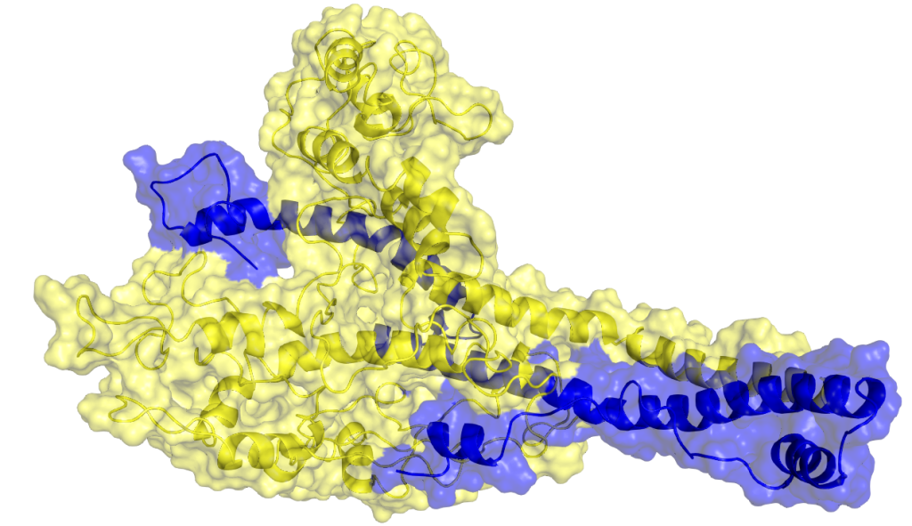
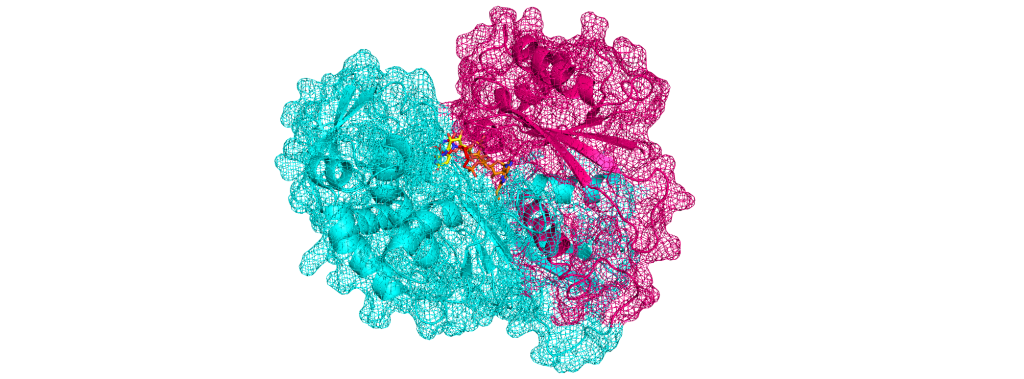
Computational Alchemy II: Diving into All Atom Molecular Dynamics Conventional Molecular Dynamics (cMD), which predominantly considers all atoms, is a powerful computational technique for simulating the motion and interactions of individual atoms within molecular systems. Developed in the 1970s and refined over decades, cMD offers unprecedented atomic-level detail, allowing researchers to study the dynamic behavior of complex biological molecules, materials, and chemical reactions with remarkable precision. By incorporating detailed force fields that describe interatomic interactions and solving Newton’s equations of motion for each atom, cMD can simulate larger systems over extended time scales. This capability provides invaluable insights into processes ranging from protein folding and drug-target interactions to materials properties and chemical reactions, making cMD an essential tool in fields such as biochemistry, materials science, and pharmaceutical research. Atomic Representation in Conventional Molecular Dynamics Models In cMD, each individual atom in a molecular system is explicitly represented and simulated. The atomic representation in cMD involves two key aspects; the level of detail in atomic modeling and the force field parameters used to describe atomic interactions. These choices directly impact the accuracy of the simulation and its computational demands. Atomic Detail and Computational Demands In cMD, the level of detail is fixed at the atomic scale, with each atom treated as a distinct particle. This granularity allows for the most accurate representation of molecular systems, capturing subtle effects such as hydrogen bonding, π-π stacking, and local electronic effects. However, this high level of detail comes at a significant computational cost. cMD simulation has to capture the spatial and temporal scales of simulations. On a spatial scale cMD needs to accurately model systems up to hundreds of thousands of atoms, (but struggles with larger systems like entire cellular organelles or material bulk properties), and on a temporal scale, it needs to capture fast atomic vibrations using time steps in the femtosecond range, limiting simulation times to nanoseconds or microseconds for most systems. Element Types and Force Fields In cMD, each atom is assigned a specific element type based on its chemical identity and local environment. These element types are crucial for defining atomic interactions. Force fields, which are sets of potential energy functions and parameters, describe the interaction parameters for different element types. They model various types of interactions, including bonded interactions (such as bond stretching, angle bending, and dihedral rotations) and non-bonded interactions (like van der Waals forces and electrostatic interactions). Biomolecular force fields, such as AMBER, CHARMM, and OPLS-AA, are optimized for proteins, nucleic acids, and other biological molecules. For a wider range of organic molecules, general-purpose force fields like GAFF and CGenFF are employed. Additionally, specialized force fields exist for inorganic systems, materials, and specific classes of compounds. The choice of force field is critical in cMD and depends on the system being studied. Selecting an appropriate force field directly impacts the accuracy and reliability of simulation results. Researchers must carefully consider their system of interest and the specific properties they wish to study when choosing a force field for their cMD simulations. Parameterization Parameterization involves assigning specific parameters to each atom and interaction in the system, ensuring that the simulation accurately represents the physical and chemical properties of the molecules being studied. This process is more complex and detailed in cMD compared to coarse-grained models due to the atomic-level resolution. Force Field Selection and Customization The foundation of parameterization in cMD is the choice of force field. Building on our introduction to force fields, the process of selecting and customizing them involves several key steps. Researchers must first evaluate available force fields based on their system of interest, reviewing literature, benchmarks, and validation studies to determine which best reproduces experimental data for similar systems. Often, a single force field may not cover all molecule types in a complex system. For instance, a protein-ligand system might require a combination of a biomolecular force field for the protein and a general-purpose force field for the ligand, necessitating careful consideration of force field compatibility. In cases where existing force fields inadequately describe certain molecular interactions, researchers may need to refine or develop new parameters. This refinement process can involve quantum mechanical calculations, fitting to experimental data, or even machine learning approaches. Atomic Charge Assignment A crucial aspect of parameterization in cMD is the assignment of partial atomic charges, which govern electrostatic interactions: Method Selection: Common methods include Mulliken population analysis, natural population analysis (NPA), and the RESP (Restrained Electrostatic Potential) method. The choice depends on the force field and the specific requirements of the system. Environment Consideration: Charges may need to be calculated for molecules in different environments (e.g., gas phase vs. solution) to accurately represent the system of interest. Charge Derivation: For novel molecules not covered by standard force fields, charges often need to be derived using quantum mechanical calculations. This process can be computationally intensive and requires expertise in quantum chemistry A protein heterodomer interaction (cMyc/Max) that was studied by utilising MD simulations. c-Myc and Max proteins are shown in yellow and blue, respectively Of course, the above discussion isn’t exhaustive. cMD parameterization often involves addressing special cases such as metal ions and post-translational modifications in biological systems. Metal ions, especially transition metals, present significant challenges due to their complex electronic structures and coordination geometries. Similarly, novel compounds, including newly synthesized molecules or those not well-represented in existing force fields, necessitate comprehensive parameterization. These cases typically require a combination of quantum mechanical calculations, experimental data fitting, and validation simulations to ensure accurate representation in cMD simulations. Modeling Interatomic Forces At the heart of cMD simulations are the interatomic forces that dictate the motion and behavior of individual atoms. Understanding these forces is crucial for interpreting simulation results and recognizing the strengths and limitations of cMD models. In contrast to coarse-grained models, cMD captures a wider range of interactions with greater detail, providing a more complete picture of molecular behavior at the atomic scale. Bonded Interactions Bonded interactions model forces between atoms directly connected by chemical
LLMs in Investment Research (III) – Summarisation of Earnings
neuralgap.io Home Sentinel Articles Home Sentinel Articles LLMs in Investment Research (III) – Summarisation of Earnings An earnings note serves as a vital tool for investors, distilling a company’s financial performance and future prospects into a concise yet comprehensive document. And more often than not, an analyst is under a lot of pressure to deliver this in a very short span of time. Crafting an effective earnings note requires a delicate balance of financial acumen, industry knowledge, and forward-thinking analysis. Even with the advent of modern LLMs, many challenges remain in supporting an analyst with the creation of these summaries. We explore the essential components of an earnings note, including key financial metrics, business highlights, management commentary, and risk factors, while also delving into the challenges LLMs face when attempting to summarize these reports. From limitations in recognizing relevant information to biases towards academic writing styles, the article examines the hurdles that must be overcome for LLMs to effectively mimic the work of experienced financial analysts. What should an Earnings Note Capture? An earnings note is a critical piece of investment research that summarizes a company’s financial performance and provides insights into its future prospects. To effectively inform investment decisions, an earnings note should generally capture the following key elements: Financial Performance Income statement, balance sheet, and cash flow-based analysis like revenue, earnings per share (EPS), and other key financial metrics Comparison to previous periods and analyst expectations Breakdown by business segments or product lines Business Highlights and Management Commentary Major achievements, milestones, or challenges during the reporting period New product launches or significant contracts Market share information CEO and CFO statements on the company’s performance Insights into the company’s strategy and future outlook Guidance and KPIs Forward-looking statements on expected performance and updates to full-year or next quarter forecasts Industry-specific metrics relevant to the company’s performance Risk Factors and Analyst Expectations Any new or evolving risks that may impact future performance How the results compare to consensus estimates Key risks to investment conclusion After-hours or pre-market trading reactions, if available Moreover, we have to keep in mind that to extract the above core points, the analyst will source information from a few key documents: Formal filings annual reports quarterly reports Earnings presentation which usually contains extra information about revenue drivers Earnings press release similarly containing key financial results and management quotes Earnings call transcript which are the verbatim record of the management’s presentation and Q&A session with analysts Supplementary financial data detailed breakdowns of financial performance, often in spreadsheet format Previous guidance and analyst estimates Relevant industry news and market conditions A point to remember is that not all notes will cover all of these details, but will tend to have several of these as relevant to the company and industry. Most importantly, research analysts who create the notes will exercise ‘recognition of relevance’ when inserting this detail into the notes. Challenges for LLMs when Creating Earnings Notes When creating an earnings summary note, a key skill an analyst exercises is the recognition of relevance of a particular bit of information and whether that piece of information should make it to the note. Analysts also focus on identifying trends, understanding the implications of financial data, and connecting current performance to future projections. Essentially, an earnings note is a summarized snapshot of the most relevant information on a company that must be optimally crafted to manage an investor’s/portfolio manager’s short attention span in conveying only the information. Subsequently, this task is also one of the most challenging for an LLM to achieve. Let’s break down the core issues as to why this is so. Multi-headed Attention Limitations: This is the mechanism which LLMs use to focus on different parts of the input simultaneously. However, this can sometimes lead to a lack of coherence in understanding the overall context. As a result, they may miss subtle but crucial connections between different pieces of information in an earnings report. For example, an LLM might fail to connect a slight decrease in profit margins with a newly mentioned supply chain disruption, whereas a human analyst would quickly make this association. Generalized Training vs. Specialized Knowledge: Most LLMs have been trained on a vast generalized space of information. While this provides them with broad knowledge, it can make it challenging to discern what’s truly relevant in a specialized field like finance. Financial relevance often requires deep industry knowledge and an understanding of market dynamics that go beyond general language patterns. An experienced analyst might recognize the significance of a minor shift in inventory levels, while an LLM might overlook this detail due to its generalized training. Context Limitation: LLMs have a maximum ‘inferable’ context, which means that even though they can process large amounts of text, they may struggle with maintaining coherence and relevance across very long documents. In practical terms, this means that information presented early in an earnings report might be ‘forgotten’ or given less weight when the model reaches the end of the document. This is particularly problematic for earnings notes, where information from the beginning (like revenue figures) needs to be held in context while processing later sections (like future guidance). Academic Writing Style Bias: LLMs often exhibit a tendency towards more academic, retrospective writing styles rather than the forward-looking, interpretive format typically employed in financial analysis. This bias stems from several factors: Training Data Composition: The training corpus frequently includes a higher proportion of academic texts, research papers, and historical analyses compared to forward-looking financial reports. Risk Aversion in Training: Many LLMs, particularly those developed by major tech companies, are trained with filters and guidelines that prioritize factual statements over speculative ones. Temporal Context Limitations: LLMs often struggle with maintaining a consistent temporal perspective, especially when asked to project future outcomes based on current data. This limitation can result in a preference for describing past events rather than extrapolating future trends. Lack of Domain-Specific Inference Training: While LLMs possess broad knowledge, they may
AI in Surveillance – Balancing Security and Privacy

neuralgap.io Dawn Articles Dawn Articles AI in Surveillance – Balancing Security and Privacy In an era where data is often hailed as the new oil, surveillance networks have become both a powerful tool for security and a source of significant privacy concerns. As organizations and governments seek to harness the benefits of widespread surveillance, they face a critical challenge: how to maintain effective monitoring while respecting individual privacy rights and complying with increasingly stringent data protection regulations. This article explores innovative approaches to this dilemma – decentralized surveillance networks with built-in data privacy safeguards. By leveraging distributed model training, secure aggregation techniques, and privacy-preserving algorithms, these systems offer a crucial way for navigating the complex landscape of security, privacy, and regulatory compliance. Distributed Processing for Enhanced Privacy and Security The foundation of decentralized surveillance networks lies in their ability to distribute the computational workload across multiple nodes. This approach not only enhances the system’s overall efficiency but also plays a crucial role in preserving data privacy. By leveraging distributed model training techniques, each surveillance node can contribute to the development of a robust, collective intelligence without the need to share raw data. This process involves local computations on individual devices or edge servers, with only model updates being shared across the network. As a result, sensitive information remains localized, significantly reducing the risk of data breaches and unauthorized access. Implementing decentralized surveillance networks with data privacy safeguards presents several technical challenges that must be addressed to ensure their effectiveness and reliability. These challenges include maintaining consistent model performance across diverse devices, managing network limitations, handling node failures, and ensuring model convergence in the face of asynchronous updates. Researchers and practitioners in the field have developed various innovative solutions to tackle these challenges, such as: Ensuring consistent model performance across heterogeneous devices Managing network latency and bandwidth constraints Handling node failures or temporary disconnections Maintaining model convergence despite asynchronous updates To implement these solutions, several algorithms and implementations have been commonly employed, including: Federated Learning: Allows models to be trained on distributed datasets without centralizing the data. It’s proposed because it maintains data locality while enabling collaborative learning. For example, Federated Averaging (FedAvg) is a popular algorithm for federated learning that averages model updates from multiple nodes. Secure Aggregation: Ensures that individual contributions to the model remain private, even from the central server. It’s crucial for preserving privacy in scenarios where model updates might inadvertently reveal sensitive information. Secure Multi-Party Computation (SMPC): One such implementation that allows multiple parties to compute an aggregate function (e.g., calculating the average or sum) over their private inputs without revealing the inputs to each other. This could be used to aggregate model updates from multiple nodes without exposing the individual updates. Differential Privacy: By adding controlled noise to the data or model updates, this method provides mathematical guarantees of privacy. It’s proposed as a way to balance utility and privacy in machine learning models. For example, Homomorphic Encryption enables computations on encrypted data, allowing nodes to contribute to the model without revealing their raw data. Example of a Real-World Scenario Let’s look at a real-world implementation of decentralized surveillance networks and examine some examples of the challenges of data privacy. Scenario: A major metropolitan area decides to implement a car mall security system that involves collaboration between local law enforcement, federal agencies, and private security firms. The goal is to enhance public safety and respond more effectively to potential threats, while ensuring the privacy of citizens and sensitive operational data. Types of Input Data: Video feeds from surveillance cameras installed throughout the car mall, capturing vehicle and pedestrian activity. License plate recognition data from entry and exit points, as well as strategic locations within the mall. Facial recognition data from cameras positioned near high-value areas or locations with increased security risks. GPS tracking data from mall security vehicles and personnel. Challenges: Ensuring the privacy and security of the collected data, as it may contain personally identifiable information (PII) of mall visitors and employees. Managing access to the data among the various collaborating agencies and firms, while preventing unauthorized use or sharing. Complying with data protection regulations and privacy laws, such as the General Data Protection Regulation (GDPR) or the California Consumer Privacy Act (CCPA). Maintaining the integrity and accuracy of the data in the face of potential tampering, hacking attempts, or system failures. Proposed Solutions to Explore: Federated Learning: Each agency or firm could train their threat detection models locally using their own data, without sharing the raw data with others. The mall’s central security system could then aggregate the model updates using techniques like Federated Averaging (FedAvg), improving the overall threat detection capabilities while keeping the input data decentralized and private. Secure Aggregation with Homomorphic Encryption: When sharing data or model updates between agencies, homomorphic encryption could be employed to allow computations on the encrypted data without revealing the underlying information. This ensures that sensitive data remains protected even during the aggregation process. Differential Privacy: To further enhance privacy, differential privacy techniques could be applied to the shared data or model updates. By introducing controlled noise, these techniques can provide mathematical guarantees of privacy, making it difficult to infer individual data points from the aggregated results. By combining these solutions, the car mall security system can leverage the power of decentralized surveillance networks while prioritizing data privacy and security. The use of federated learning and secure aggregation allows for collaborative threat detection without compromising individual agency data, while differential privacy adds an extra layer of protection. Robust access control and data governance measures ensure that the collected data is used responsibly and in compliance with relevant regulations. We help enterprises build competitive advantage in AI Neuralgap helps enterprises build very complex and intricate AI models and agent architectures and refine their competitive moat. If you have an idea – but need a team to iterate or to build out a complete production application, we are here. Please enable JavaScript in your browser to
Computational Alchemy: Leveraging Structure-Based Virtual Screening and ML Scoring
Leveraging Structure-Based Virtual Screening and ML Scoring Computational Alchemy In the relentless pursuit of novel therapeutics, computational methods have become indispensable tools in modern drug discovery. The ultimate goal of Structure-Based Virtual Screening (SBVS) and Machine Learning-based (ML) scoring is to accelerate the drug discovery process by efficiently identifying promising lead compounds that can bind strongly and selectively to a target protein, reducing the time and cost associated with experimental screening and validation. SBVS and ML scoring are complementary approaches that, when used in combination, can enhance the efficiency and effectiveness of the drug discovery pipeline. SBVS enables the rapid exploration of vast chemical spaces by virtually “docking” large libraries of compounds into the binding site of a target protein, while ML scoring refines and re-scores these docked poses to identify the most promising candidates. In this article, we will explore the principles behind these computational techniques, their advantages, and how they are being applied to tackle the challenges of finding new drug candidates in an increasingly complex and data-rich landscape. Structure-Based Virtual Screening: Navigating the Vast Chemical Space Structure-Based Virtual Screening (SBVS) is a powerful computational approach that allows researchers to navigate the vast chemical space in search of potential drug candidates. By leveraging the 3D structure of a target protein, SBVS enables the virtual “docking” of large libraries of compounds into the protein’s binding site to evaluate their potential to form favorable interactions. This process involves assessing the structural complementarity between the ligand and the protein, as well as estimating the strength of their intermolecular interactions. A typical SBVS workflow begins with the preparation of the target protein structure, often obtained through experimental techniques such as X-ray crystallography or NMR spectroscopy. The protein structure is then optimized for docking by adding hydrogen atoms, removing water molecules, and defining the binding site region. Next, a large library of small molecules, known as ligands, is prepared by generating 3D conformations and assigning appropriate protonation states and partial charges. In recent years, the size of these libraries has exploded, with leading commercial sources like Enamine REAL, WuXi GalaXi, and Otava CHEMriya now offering a combined total of over 50 billion compounds, a staggering 2000-fold increase in just a decade. The core of SBVS lies in the docking process, where each ligand from the library is systematically placed into the protein’s binding site, and its orientation and conformation are optimized to achieve the best fit. Docking algorithms employ various search strategies, such as exhaustive search, genetic algorithms, or Monte Carlo methods, to explore the conformational space of the ligand within the binding site. The quality of the ligand pose is evaluated using a scoring function that estimates the binding affinity between the ligand and the protein. Scoring functions can be based on physical principles, such as force fields or empirical energy terms, or they can be knowledge-based, derived from statistical analysis of known protein-ligand complexes. However, the accuracy of these scoring functions remains a significant challenge, with physics-based methods often being too computationally expensive for large-scale screening and empirical methods struggling to capture the full complexity of protein-ligand interactions. Despite these limitations, SBVS has proven to be a valuable tool in drug discovery, enabling the rapid screening of millions of compounds, filtering out unlikely candidates, and prioritizing those that are most likely to bind to the target protein. This approach significantly reduces the number of compounds that need to be synthesized and tested experimentally, saving time and resources in the early stages of drug discovery. Recent studies have demonstrated hit rates as high as 33% using advanced techniques like V-SYNTHES and 39% with Chemical Space Docking, compared to hit rates of around 15% for standard virtual screening approaches, showcasing the potential of SBVS in identifying promising drug candidates. ML Scoring Post-SBVS: Refining the Chemical Space for Lead Discovery Once the SVBS has been successfully completed, ML-based is the next phase of the drug discovery pipeline. After the initial docking process in SBVS, where large libraries of compounds are screened and their poses optimized in the protein’s binding site, ML scoring can be used to refine and re-score the docked poses. This approach helps to filter out false positives that may have been scored favorably by traditional scoring functions but are less likely to bind strongly to the target in reality. The implementation of ML-based scoring functions has shown significant performance improvements over traditional methods. Studies have demonstrated that ML scoring functions can achieve moderately strong correlations between predictions and experimental binding affinities, with Pearson correlation coefficients (Rp) ranging from 0.55 to 0.60 for experimental and computer-generated databases, respectively. This represents a substantial improvement over classic scoring functions, which in some cases only achieve Rp values of around 0.2. Furthermore, ML-based scoring functions have demonstrated superior speed by being several orders of magnitude faster than traditional scoring functions. This combination of improved accuracy and speed makes ML scoring a powerful tool for refining SBVS results and identifying the most promising lead compounds. Different types of ML scoring mechanisms have been explored, each with its own strengths and limitations. One crucial distinction is between horizontal and vertical testing protocols. Horizontal tests, where proteins may be present in both training and test sets (albeit with different ligands), tend to yield overly optimistic results due to similarities between training and test data. Vertical tests, where test proteins are entirely excluded from the training set, provide a more realistic assessment of performance in real-world scenarios. Recent studies have also explored the potential of per-target scoring functions, which are trained on computer-generated databases specific to individual proteins. These per-target models have shown promising results, achieving average Rp scores of 0.44-0.52, compared to 0.30 for universal scoring functions in vertical tests. This suggests that tailoring ML scoring functions to specific targets could significantly enhance their predictive power. Nevertheless, despite the advancements in ML-based scoring, several challenges still remain. One significant issue is the need for explicit protein-ligand interaction data, which can be computationally expensive and time-consuming to generate.